Graph View

Clicking displays the graph view. Click this button again to close the graph view. The graph view is divided into two areas: the CCDF plot on the left side and the waveform plot on the right side. A waveform can only be plotted after it has been generated.

CCDF Plot

The complementary cumulative distribution function (CCDF) plot displays the generated waveform's calculated peak-to-average power ratio (measured in dB) along a scale of percent probability. The table to the left of the CCDF plot displays the calculated peak-to-average values for the current waveform, which is the yellow curve. For additional information, see Understanding CCDF Curves.

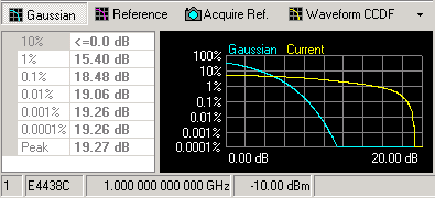
In addition to the waveform's current plot (yellow), up to three previous plots are also displayed in shades of gray, allowing you to make comparisons of waveform characteristics as you adjust parameters. You can also designate a reference curve (red).

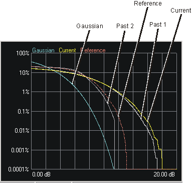
Click this button to toggle the band-limited Gaussian noise reference curve (blue) on or off.

Click this button to toggle the reference curve (red) on or off.

Click this button to make the current waveform curve (yellow) the reference curve (red).

From the drop-down window, select Waveform CCDF or Burst CCDF to select the portion of the waveform used to calculate the CCDF data. Waveform CCDF will include all components of the configured frame including gaps and non-transmitted portions (both RF burst on and off portions). Burst CCDF will include the configured bursts only (not including gaps or times when the RF burst is off).

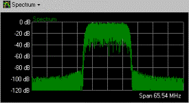
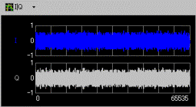
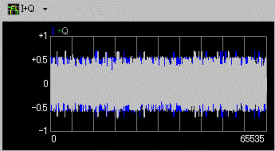
Waveform Plot

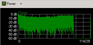
Click this button to select from the list of different waveform plots. Selections include Power (shown above), I+Q, I|Q, and Spectrum. Each click selects the next plot type in the list. You can also click the arrow to access a drop-down menu where you can make a direct selection. If the total number of points exceeds 64000, the first 64000 points are shown.