Time Averaging

Unlike other average types, Time averaging is done in the time domain, as shown in the following block diagram. Notice that time averaging is performed before the FFT Fast Fourier Transform: A mathematical operation performed on a time-domain signal to yield the individual spectral components that constitute the signal. See Spectrum..

$image\blk_maintime_wmf.jpg$

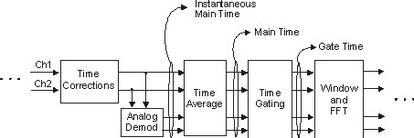
This block diagram is a portion of the Vector and Analog Demodulation block diagrams. Click the following links to see the entire block diagrams:
Vector Signal Analysis Block Diagram

Analog Demodulation Block Diagram

Time corrections are shown in the previous block diagram for completeness; however, time corrections are not required to perform time averaging.

With time averaging, the VSA averages "N" time records (where "N" is the number of averages) and then stops. Use Restart to repeat the process.

When using specific hardware (like the X Series Analyzers), can affect time averaging and should be turned off (, clear check box).

Although measurements made with time averaging have better signal-to-noise ratios than rms averaging, there are some restrictions:

The input signal must be periodic. In other words, the frequency components to measure must repeat with each time record. If these components are not periodic (they do not maintain the same phase relationship), their real and imaginary values will cancel and the VSA will not resolve these components.
When time averaging is selected, an external trigger signal will need to be provided. Of course, the VSA will still make a measurement with free run triggering (no trigger signal), but the amplitude of periodic signals will diminish with each successive average (because even periodic components have random phase with free run triggering).

For averaging formulas, see the help for the type of trace data selected. For example, refer to the help topic for the Spectrum trace, which includes formulas that show how the VSA creates averaged spectra. Also, most measurement types' Error Summary traces topics contain some information about supported averaging types.

Time Averaging and Time Records

With time averaging, the VSA makes trigger corrections so a stable time record can be viewed.

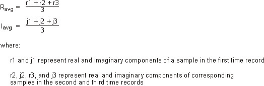
With time averaging, real and imaginary components are averaged separately. For example, if the number of averages is 3:

$image\r1j1Formula_wmf.jpg$