How DSP Cross-Correlation Removes Measurement Errors

Here is a simple explanation of how DSP cross-correlation removes measurement errors. It is simplified in that it describes the computation of the standard deviation of a random variable, C, in the presence of measurements errors, A and B. The oscilloscope's actual calculations of Time Interval Error (TIE) and phase noise are slightly more complicated, but the noise reduction mechanism is the same.

Consider a random variable, C, of which we want to determine its standard deviation.

The standard deviation of C is the square root of the variance of C:

Because the standard deviation is directly related to variance by a square root function, this explanation will refer only to the variance calculation and leave the conversion to standard deviation to the reader. To simplify the formulas, this explanation will also assume all random variables have a zero mean.

Ideally, we would measure a set of individual values of C and then compute its variance using the following formula:

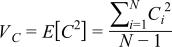
The variance of C is equal to the expected value of C squared or the mean of C squared:

In reality however, we cannot measure C directly because our measurement device adds its own error, A. So, all we get to know is the variance of C+A. Given the measured values, M=C+A, the formula below shows how the presence of A corrupts our desired measurement of C.

The variance of the measured values is the variance of C+A:

Consider the three terms in the right-hand portion of the above equation when C and A are uncorrelated to each other. The first two terms,

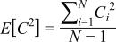
and

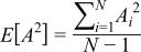
both sum to positive, non-zero values because A2 and C2 are always positive, non-zero values. The last term,

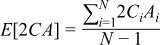
however, sums to zero because A and C do not always have the same sign and the sum of their product eventually approaches zero with an increasing number of measurements. So, when C and A are uncorrelated, the variance of their sum becomes:

The variance of the sum of two uncorrelated random variables is equal to the sum of their variances:

Now, consider measuring C using two independent measurement devices. One device adds an uncorrelated random error, A, and the other device adds an uncorrelated random error, B. This time, use the following equation to compute the variance of C.

Variance calculation method used by the two-channel cross-correlation noise reduction technique:

In this case, all three error terms in the right-hand portion of the equation above average to zeros, leaving only the desired error-free variance of C.

The uncorrelated errors from the two independent measuring devices average to zero, leaving only the variance of C:

Note that this noise reduction technique does not remove all the error instantly, but rather reduces the error with increasing sample size, in the same way that averaging does. This means that there can be a measurement accuracy versus measurement time trade-off. If necessary, you can increase the number of waveform acquisitions or increase the waveform record size to reduce the oscilloscope's residual uncorrelated noise. Every 10-times increase in the amount of measurement data analyzed will reduce the uncorrelated errors by another -5 dB.