Other topics about Analysis and Processing of Result
Equation Editor allows you to enter an algebraic equation of standard mathematical operators and functions, referencing data that is available in the E4990A. Once a valid equation is entered and enabled, the display of the active trace is replaced with the results of the equation, and updated in real-time as new data is acquired. For equations that can be expressed with Equation Editor's supported functions, operators, and data, there is no need for off-line processing in a separate program.
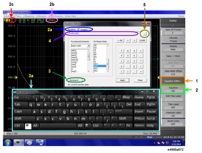
For example, on entering the equation "Z=ACV/ACI" in the E4990A Equation Editor (2c in the Figure below), the resulting trace is computed as each ACV data divided by ACI, that resulting trace is as same as absolute Z. For a 201 point sweep setup, the computation is repeated 201 times, once for each point.
The step-by-step procedure of using Equation Editor is described below:
Select a trace in which you want to enter the equation and activate the trace.
Activating a trace is required as Equation Editor works on traces.
Follow the steps below to enter an equation:
Press Display.
Click Equation Editor (1 in the figure above). The Equation Editor dialog box appears.
Enter an equation in the equation field (4 in the figure above).
Referring to traces in a different channel is NOT available with Equation Editor on the E4990A.
The equation can be entered with the software keyboard enabled by selecting Keyboard... (3 and 3a in the figure above).
Follow the steps below to apply the defined equation. When a valid equation is entered, the Equation Enabled check box becomes available for checking.
Check Equation Enabled (√) check box (2a in the figure above).
Click Apply. The equation becomes visible and annotation of [Equ] (2b in the figure above) is displayed in the trace title area.
Click Close to hide the dialog box.
The equation can also be applied by selecting Display > Equation [ON] (2 in the figure above).
If error correction is not turned ON, then the raw, uncorrected data is used in the equation trace.
As for E4990A, an equation is always valid.
The data trace of measured channel is always measured in E4990A. The equation might be invalid when referring to a memory trace and the memory trace isn't displayed.
The following examples may help you in getting started with Equation Editor. Input the equation example in the equation field (4 in Equation Editor dialog box).
|
Description |
Parameter |
Equation Example |
|
Add 50 Ω offset on Trace 1 |
Z |
Offset=data(1)+50 |
See the internal data processing for equation editor data processing position.
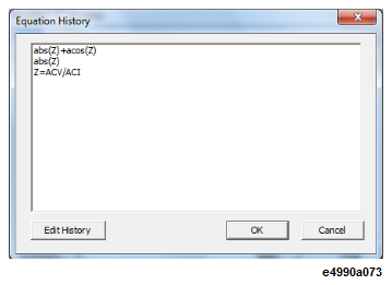
Equation Editor has the capability to save and recall all previously defined equations. All equations can be viewed in the Equation History dialog box.
To view the equations in the list, follow this procedure:
Open Equation Editor by Display > Equation Editor.
Enter an equation and click Apply in the Equation Editor Dialog box to save the defined equation in the directory of the E4990A. To view a list of saved equations, click the ... button (5 in Equation Editor Dialog box) to open the Equation History dialog box.
To store an equation in the History List, the equation must be applied first. This can be done by clicking on the Apply button.
To edit the equations in the list, click Edit History. The text file of history list is opened with Notepad.
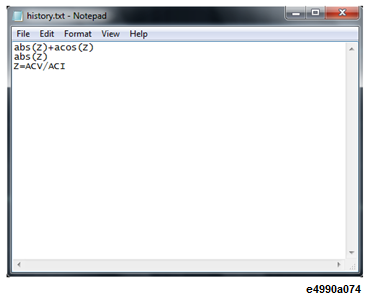
The History List is stored as a text file D:\Agilent\Equation\history.txt and can save a maximum of 50 lines (equations) with a maximum of 254 characters per line (equation).
The following table describes the different functions and constant available in the E4990A Equation Editor. In the following table:
Function(scalar x) means that the function requires a scalar value. If a complex value is entered, it is automatically converted to a scalar value; complex(x,y) -> scalar(x)
Function(complex x) means that the function requires a complex value. If a scalar value is entered, it is automatically converted to a complex value; scalar(x) -> complex(x, 0)
a,b are arguments that are used in the function.
Basic Math Functions
|
Function |
Description |
|
abs(complex a) |
returns the sqrt(a.re2+a.im2) |
|
acos(scalar a) |
returns the arc cosine of a in radians |
|
asin(scalar a) |
returns the arc sine of a in radians |
|
atan(scalar a) |
returns the arc tangent of a in radians |
|
atan2(complex a) |
returns the phase of a = (re, im) in radians |
|
atan2(scalar a, scalar b) |
returns the phase of (a, b) in radians |
|
conj(complex a) |
returns the conjugate of a |
|
cos(complex a) |
takes a in radians and returns the cosine |
|
cpx(scalar a, scalar b) |
returns a complex value (a+ib) from two scalar values |
|
exp(complex a) |
returns the exponential of a |
|
im(complex a) |
returns the imaginary part of a as the scalar part of the result (zeroes the imaginary part) |
|
ln(complex a) |
returns the natural logarithm of a |
|
log10(complex a) |
returns the base 10 logarithm of a |
|
mag(complex a) |
returns sqrt(a.re2+a.im2) |
|
phase(complex a) |
returns atan2(a) in degrees |
|
pow(complex a,complex b) |
returns a to the power b |
|
re(complex a) |
returns the scalar part of a (zeroes the imaginary part) |
|
sin(complex a) |
takes a in radians and returns the sine |
|
sqrt(complex a) |
returns the square root of a, with phase angle in the half-open interval (-π/2, π/2) |
|
tan(complex a) |
takes a in radians and returns the tangent |
|
Constants |
|
|
e |
2.71828182845904523536 |
|
PI |
3.14159265358979323846 |
Mutual transformation is automatically made for scalar and complex.
scalar(x) -> complex(x,0)
complex(x,y) -> scalar(x)
|
Operator |
Description |
|
+ |
Addition |
|
- |
Subtraction |
|
* |
Multiplication |
|
/ |
Division |
|
^ |
Power |
|
( |
Open parenthesis |
|
) |
Close parenthesis |
|
, |
Comma - separator for arguments |
|
= |
Equal (optional) |
|
E |
Exponent (as in 23.45E6) |
Priority of operators is:
^
*, /
+, -