The SRL feature is designed to measure cable impedance and structural return loss. Cable impedance is the ratio of voltage to current of a signal traveling in one direction down the cable. Structural return loss is the ratio of incident signal to reflected signal in a cable, referenced to the cable's impedance.
The network analyzer uses a synthesized RF signal source to produce an incident signal as a stimulus. A reflection measurement is made and then used to compute the cable impedance. The structural return loss measurement is displayed referenced to the measured cable impedance.
For CATV cable, the cable is measured from 5 MHz to 1000 MHz at narrow frequency resolutions down to 125 kHz. The analyzer, with a furnished VBA utility program, automatically scans the cable, then reports the worst-case responses.
The following items are described in this topic.
Other topics about Structural Return Loss Measurement
The analyzer automatically computes the cable impedance (Z). However, if you wish to turn OFF this "auto Z" function and input your own value of impedance, you can. See Connector Model for Short Cables.
In coaxial cable, the value of the impedance depends upon the ratio of the inner and outer conductor diameters, and the dielectric constant of the material between the inner and outer conductors. The cable impedance is also affected by changes in conductivity. These changes are a natural consequence of RF currents that flow near the surface of a conductor. This effect is known as the "skin effect." Also, the construction of the cable can change along the length of the cable, with differences in conductor thickness, dielectric material and outer conductor diameter changing due to limitations in manufacturing. Thus the cable impedance may vary along the length of the cable.
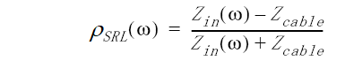
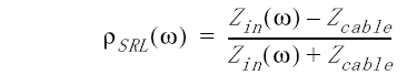
The extent to which manufacturing imperfections degrade cable performance is characterized by a specification called structural return loss (SRL). SRL is the ratio of incident signal to reflected signal in a cable. This definition implies a known incident and reflected signal. In practice, the SRL is loosely defined as the reflection coefficient of a cable referenced to the cable's impedance. The reflection seen at the input of a cable, which contributes to SRL, is the sum of all the tiny reflections along the length of the cable. In terms of cable impedance, the SRL can be defined mathematically as:
Equation 1
Zin is the impedance seen at the input of the cable, and Zcable is the nominal cable impedance.
Cable impedance is a specification that is defined only at a discrete point along the cable, and at a discrete frequency. However, when commonly referred to, the impedance of the cable is some average of the impedance over the frequency of interest. Structural return loss, on the other hand, is the cumulative result of reflections along a cable as seen from the input of the cable. The above definitions need to be expressed in a more rigorous form in order to apply a measurement methodology.
Following are three common methods of defining cable impedance. Although all three methods may be commonly used in your industry, your network analyzer uses the third method (Z-average normalization) to define cable impedance.
One definition of cable impedance is that impedance which results in minimum measured values for SRL reflections over the frequency of interest. This is equivalent to measuring a cable with a return loss bridge that can vary its reference impedance. The value of reference impedance that results in minimum reflection, where minimum must now be defined in some sense, is the cable impedance. Mathematically, this is equivalent to finding a cable impedance such that:
Equation 2
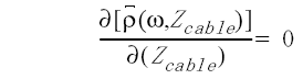
where ρ is some mean reflection coefficient. Thus, cable impedance and SRL are somewhat inter-related: the value of SRL depends upon the cable impedance, and the cable impedance is chosen to give a minimum SRL value.
An alternate definition of cable impedance is the average impedance presented at the input of the cable over a desired span. This can be represented as:
Equation 3
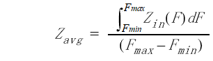
The value found for Zavg would be substituted for Zcable in Equation 1 to obtain the structural return loss from the cable impedance measurement.
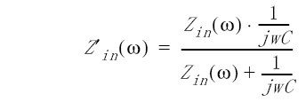
The mathematics for the Z-average normalization as performed by the analyzer are shown below.
Equation 4
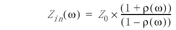
Z0 = system impedance, 50 Ω.
Equation 5
Equation 6
In Equation 4, ρ(ω) is the reflection coefficient from the analyzer measured at each frequency and Zin(ω) is the impedance of the cable for that measured reflection coefficient.
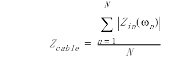
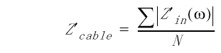
The calculation of Zcable, described in Equation 5, is the Z-average impedance of the cable over the number of frequency points (N). The default frequency range is approximately 5 MHz to 200 MHz. This frequency range is chosen because mismatch effect of the input connector is small. High quality connectors must be used if the average impedance is calculated over a wider span. The frequency range for this calculation can be modified by using the Z Cutoff Freq. softkey in the connector model menu to change the cable impedance cutoff frequency.
Equation 6 is the structural return loss for the cable. This calculation can be done by the analyzer or an external computer.
SRL is the measurement of the reflection of incident energy that is caused by imperfections or disturbances (bumps) in the cable which are distributed throughout the cable length. These bumps may take in the form of a small dent, or a change in diameter of the cable. These bumps are caused by periodic effect on the cable during the manufacturing process. For example, consider a turn-around wheel with a rough spot on a bearing. The rough spot can cause a slight tug for each rotation of the wheel. As the cable is passed around the wheel, a small imperfection can be created periodically corresponding to the tug from the bad bearing.
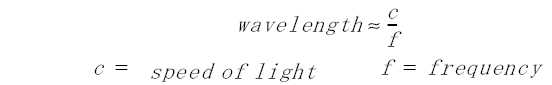
Each of these small variations within the cable causes a small amount of energy to reflect back to the source due to the non-uniformity of the cable diameter. Each bump reflects so little energy that it is too small to observe with fault location techniques. However, reflections from the individual bumps can sum up and reflect enough energy to be detected as SRL. As the bumps get larger and larger, or as more of them are present, the SRL values will also increase. The energy reflected by these bumps can appear in the return loss measurement as a reflection spike at the frequency that corresponds to the spacing of the bumps. The spacing between the bumps is one half the wavelength of the reflection spike and is described by equations 7 and 8.
Equation 7
Equation 8

The wavelength/2 spacing corresponds to the frequency at which down and back reflections add coherently (in-phase). The reflections produce a very narrow response on the analyzer display that is directly related to the spacing of the bumps. The amount of reflected energy is observed as return loss. When this return loss measurement is normalized to the cable impedance, the return loss becomes structural return loss.
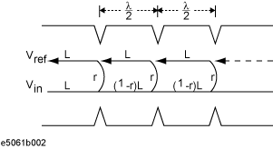
The following figure diagrams reflections from bumps in a cable. We can combine the energy reflected by each bump in a cable and make a few basic assumptions, to mathematically describe SRL with the series shown in Equation 9.
Equation 9
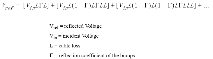
The bumps are assumed to be uniform in reflection and spaced by a wavelength/2 separation.
The series may be reduced to a simple form to leave us with the relationship shown in Equation 10. The term L is a function of the loss of the cable at a specific frequency and the wavelength at that frequency.
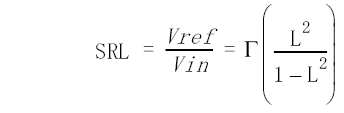
The term (L2)/(1-L2) can be thought of as the number of bumps that are contributing to SRL. It represents a balance between the contribution of loss in a single bump and further bumps in the cable for the specified frequency and cable loss. Calculate the distance into the cable by multiplying the term (L2)/(1-L2) by the distance between bumps.
The following table illustrates some calculated values for a typical trunk cable. From the table, bumps spaced 1.5 meters apart out to 307 meters contributes to SRL.
|
Frequency |
Spacing (λ/2)m |
Loss (dB)/m |
dB/bump |
bumps |
Distance (m) |
|
100 MHz |
1.5 |
0.014 |
-0.02 |
205 |
307 |
|
500 MHz |
0.3 |
0.033 |
-0.01 |
433 |
129 |
|
1 GHz |
0.15 |
0.05 |
-0.0075 |
554 |
83 |
Refer to Periodic Bumps in a Cable and Equation 10 for the following discussion.
Γ = the reflection coefficient of each bump (Vreflected/Vincident)
L = the cable loss between bumps (Vtransmitted/Vincident)
The distance between bumps equals λ/2 (1/2 wavelength).
Typical values:
Γ << 1
L ≤ 1 for low loss cable
In Equation 10, L is the cable loss for a 1/2 wavelength length of cable, expressed in linear.
Find the cable loss from a spec sheet. Cable loss is typically expressed in loss per foot.
Convert loss per foot to loss per meter.
Find the 1/2 wavelength in meters. This will be the spacing between bumps.
Multiply loss per meter × 1/2 wavelength to get dB loss per bump.
Convert dB loss per bump to linear.
A spec sheet states that the cable loss spec at 300 MHz is 1 dB per 100 feet.
Convert loss per foot to loss per meter:
1 dB/100 ft ≈ 1 dB/30 m ≈ 0.033 dB/m
This is the Loss (dB)/m column in SRL Equation Constant.
Find the 1/2 wavelength in meters:
1/2 wavelength at 300 MHz ≈ 0.5 meters
This is the Spacing (λ/2)m column in SRL Equation Constant.
Multiply loss/meter × 1/2 wavelength:
0.033dB/meter × 0.5 meters = 0.0165 dB = LdB
This is the dB/bump column in SRL Equation Constant.
Convert LdB (loss) in dB to linear:
20 log (LdB) = -0.0165 L = 10(-0.016/20) = 0.998
(L2)/(1-L2) ≈ 262
There are approximately 262 bumps contributing to SRL at 300 MHz.
262 × 0.5 = 131. The distance into the cable for 262 bumps is 131 meters.
In actual cables, the reflections from the bumps and the spacing of the bumps may vary widely. The best case for a minimum SRL, is that the bumps are totally random and very small. Real world examples are somewhere in between the uniform bumps and scattered case. As the sizes of the bumps, their spacing, and the number of bumps vary within the manufacturing process, varying amounts of SRL are observed.
In addition to a set of periodic bumps, a cable can also contain one or more discrete faults. For this discussion, discrete imperfections is referred to as “faults,” and periodic imperfections is referred to as "bumps."
Reflections from discrete faults within the cable also increases the level of SRL measured. The energy reflected from a fault sums with the energy reflected from the individual bumps and provide a higher reflection level at the measurement interface. Examining the cable for faults before the SRL measurement is a worthwhile procedure. The time required to perform the fault location measurement is small compared to the time spent in performing an SRL measurement scan.
A fault within the cable provides the same type of effect as a bad connector. If the fault is present within the end of the cable nearest to the analyzer, the effect is noticed throughout the entire frequency range. As the fault is located further into the cable, the cable attenuation reduces the effect at higher frequencies. The reflected energy travels further through the cable at lower frequencies where the cable attenuation per unit distance is lower.
To remove the unwanted effects of worn connectors, the SRL measurement uses a built-in connector model. The connector model consists of compensation for connector length and compensation for connector capacitance (connector C).
The "connector C" compensation emulates the C trim value of a variable impedance bridge.
The connector length is used to compensate for the effects of an electrically long connector and extends the calibration reference plane.
A calibration reference plane is established at the point where the short, open, and load standards are measured.
The analyzer can automatically measure the optimum values for your connector model, or you may enter them manually.
The default values for the connector model are 0.00 mm length, and 0.00 pF capacitance (no compensation).
When measuring spools of the cable, typically two connectors are used: the test-lead connector and the termination connector. (See the following figure.) These connectors provide the cable interface and are measured as part of the cable data.
Basic SRL Measurement Setup and Connections
Often, slight changes in the test-lead connector can cause significant changes in the values of structural return loss measured at high frequencies. This is because the reflection from a connector increases for high frequencies. In fact, the return loss of a test-lead connector can dominate the SRL response at frequencies above 500 MHz. This is where training, good measurement practices, and precision cable connectors are needed, especially for measurements up to 1 GHz. Precision connectors are required to provide repeatability over multiple connections. Slip-on connectors are used to provide rapid connections to the cables, but require careful attention in obtaining good measurement data. Repeatability of measurement data is directly affected by the connector's ability to provide a consistently good connection. This is the major cause of repeatability problems in SRL measurements.
Effects of the test-lead connector at the measurement interface are observed as a slope in the noise floor at higher frequencies.
By observing the SRL measurement display and slightly moving the connector, the effects of the connection can be observed at the higher frequencies. The test-lead connector should be positioned to obtain the lowest possible signal level and the flattest display versus frequency. The mechanical interface typically provides an increasing slope with frequency and flattens out as the connection is made better.
The termination connector may also affect the SRL measurement if the cable termination connector and load provide a significant amount of reflection and the cable is short enough. As longer lengths of cable are measured, the cable attenuation provides isolation from the termination on the far end. Use a fault location measurement technique to observe the reflection from the termination at the far end of the cable. If the termination is shown as a fault, the reflection from the terminating connector is contributing to the reflection from the cable. A more suitable termination is required or a longer section of cable must be measured. The cable must provide sufficient attenuation to remove the effects of the connector and load for a good SRL measurement. Performing a good measurement on a short length of cable is quite difficult and requires connectors with very low reflections to be effective.
The analyzer employs the fixed-bridge method and instrument software to emulate the traditional variable-bridge method. Vector error correction is used to provide the most accurate measurements up to the calibration plane defined by the calibration standards. Additional corrections can also be used to minimize the effects of the test-lead connector on the measured SRL response.
The error corrections done for a fixed bridge can also include connector compensation. The fixed bridge method with connector compensation technique mathematically removes the effects of the test-lead connector by compensating the predicted connector response given by a connector model.
One model that can be used for the cable connector is the shunt C connector model. With this model, the adjustment of the C value given in a variable impedance bridge can be emulated. The shunt C connector model assumes the discontinuity at the interface is abrupt and much smaller than a half wavelength of the highest frequency of measurement. With this assumption, the discontinuity can be modeled as a single-shunt twisted pair, where C = C0 + second and third order terms.
Intuitively this is the right model to choose because the effect of a typical poor connector on structural return loss measurement is an upward sloping response, typically worst at the high frequencies.
Using a shunt C to model the connector, a value of the susceptance, -C, may be chosen by the network analyzer to cancel the equivalent C of the connector and mathematically minimize the effect of the connector on the response measurement.
The equations for computing structural return loss and the average cable impedance with capacitive compensation are described next.
Equation 11
Equation 12
Equation 13
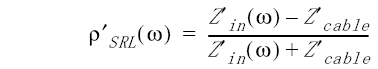
In Equation 11, Zin(w) is calculated from the measured return loss as described in Equation 4, previously. The primed values are the new calculation values using the capacitive compensation. With these equations, the network analyzer can compute values for the cable impedance and mathematically compensate for the connector mismatch with a given value of C connector compensation.
The shunt C connector model can be improved with the addition of connector length. Connector length is used to compensate the phase shift caused by the electrical length within the connector. The calibration plane can be moved from one side of the cable connector to the other side, so that the shunt C is placed exactly at the discontinuity of the connector and cable under test.
In any comparison of cable impedance or structural return loss data, it is important to understand the measurement uncertainty involved in each type of measurement. This is critical for manufacturers, who often use the most sophisticated techniques to reduce manufacturing guard bands. It is also important in field measurements that users choose the proper equipment for their needs, and understand the differences that can occur between manufacturers’ data and field data. Also, note that measurement uncertainty is usually quoted as the worst-case result if the sources of error are at some maximum value. This is not the same as error in the measurement, but rather a way to determine measurement guard band, and to understand how closely to expect measurements to compare on objects measured on different systems.
The errors that can occur in a reflection measurement are reflection tracking (or frequency response), T, source match, ΓM, and directivity, D. The total error in a measurement can be shown to be
Equation 14
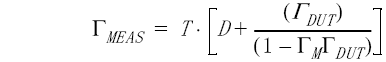
where ΓDUT is the reflection response of the DUT.
Error correction techniques can effectively remove the effects of tracking. Also, source match effects are small if ΓDUT is small. This leaves directivity as the largest error term in the reflection measurement. The causes and effects of these error terms will be described for each of the measurement methodologies.
For variable bridge measurements, the directivity of the bridge is the major error term. One-port vector error correction reduces the effects of tracking and source match, and improves directivity. The directivity after error correction is set by the return loss of the precision load, specified to be better than 49 dB at 1 GHz. However, the directivity is only well known at the nominal impedance of the system, and the directivity at other impedances should be assumed to be that specified by the manufacturer. For best performance, the bridge should be connected directly to the cable connector, with no intervening cable in between.
The directivity of the bridge could be determined at impedances other than 75 ohms, by changing the impedance and measuring the resulting values. This can be done by changing the reference impedance to the new value, say 76 ohms, changing the bridge to that value, and measuring the impedance on a Smith chart display. The difference from exactly 75 ohms represents the directivity at that impedance.
For fixed bridge methods, the reflection port is often connected to the cable connector through a length of test lead. A one-port calibration is performed at the end of the test lead. The directivity is again set by the load, but any change in return loss of the test lead due to flexing degrades the directivity of the measurement system. In both fixed and variable bridge measurements, the repeatability and noise floor of the analyzer may limit the system measurement. A convenient way to determine the limitation of the measurement system is to perform a calibration, make the desired measurement, then re-connect the load to check the effective directivity. A very good result is better than -80 dB return loss of the load. Typically, flexure in the test leads, connector repeatability, or noise floor in the network analyzer limits the result to between -60 to -40 dB. If the result is better than -49 dB, then the system repeats better than the load specification for the best available 75 Ω loads. Thus, the effective directivity should be taken to be the load spec of -49 dB. It is possible to reduce this limitation by having loads certified for better return loss.
The fixed bridge method calculates the cable impedance by averaging the impedance of the cable over frequency. The variable bridge uses a reading of the impedance from the dial on the bridge. The directivity at any impedance can be determined, as stated earlier, but only to the limit of the return loss of the load, and the system repeatability.
Any connectors and adapters used to connect the test-lead cable to the cable under test can have a significant effect on the impedance measurement. With the variable bridge method, the operator determines the appropriate setting, taking into account the capacitive tuning adjustment. With the fixed bridge method, it is also possible to compensate somewhat for the connector. However, it is often the case that the cable impedance is determined by the low frequency response, up to perhaps 200 MHz to 500 MHz, where the connector mismatch effect is still small. The choice of frequency span to measure cable impedance can itself affect the value obtained for cable impedance. In general, as the connector return loss becomes worse, it has a greater effect on the resulting impedance measurement. The uncertainty caused by the connector is difficult to predict, but large errors could occur if the low frequency return loss is compromised to achieve better high frequency structural return loss.
Finally, note that since both methods average, in some way, the measurement over the entire frequency range, it is probable that the worst case error will never occur at all frequencies, and with the same phase. In fact, it is more likely that the errors will cancel to some extent in cable impedance measurements. Also, the loads that are used will invariably be somewhat better than specified, especially over the low frequency range.
The same factors that affect cable impedance - directivity, system and test lead stability, and cable connector mismatch - also affect structural return loss. However, since structural return loss is measured at all frequencies, it is much more likely that a worst case condition can occur at any one frequency. For that reason, the measurement uncertainty must include the full effect of the above listed errors.