MATLAB® Equations


Beginning with PLTS 2012, a runtime version of MATLAB is installed with PLTS. This allows PLTS to use MATLAB capabilities 'behind the scenes'. In addition, you can also write your own MATLAB functions and use them in PLTS from the following dialog.

Note: Beginning with PLTS 2018, the full version of MATLAB is NOT required to use PLTS capability. See the MATLAB website at:http://www.mathworks.com/products/matlab/index.html

In this topic:

How to call a MATLAB Equation from PLTS

  1. Click Tools, then Math, then Collaborate with MATLAB

Create Equations dialog box help

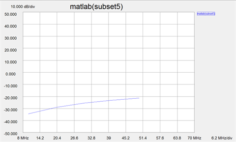
See Example of how to use this feature.

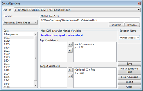
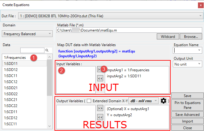
In this dialog, you specify the parameters to send to the MATLAB function, and the variable name in which the resulting data will be stored.

Matlab File - Navigate to a *.m file which contains the variables to be mapped to data.

Note: There can be NO spaces in the entire path name of the MATLAB *.m file.

Domain - Choose the domain data to map. Select from Frequency Domain (single-ended and balanced) and Time Domain (single-ended and differential).

Data - Click a parameter, then click a variable, then click >> to associate the data with the variable.

Equation Name - Enter a name to save the equation and recall it for future use.

Output Unit - Set the output units to No unit,  Ohms, or dB.

Wildcard - Replaces file number with '?' when the file number is not the same as when the equation was first written.

Browse - Specifies the path to the *.m MATLAB file.
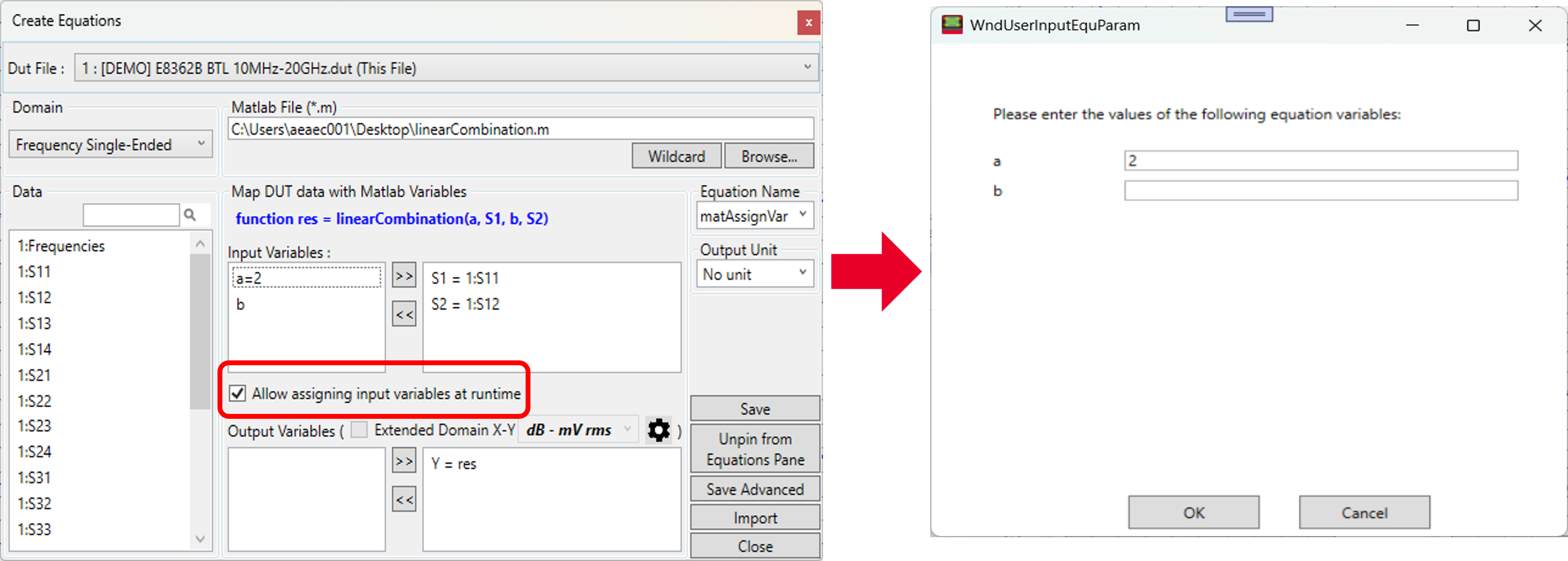
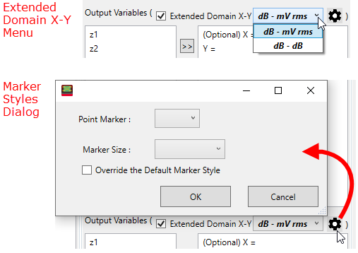
Extended Domain X-Y - Mark the checkbox to enable the X-Y units selection from the drop-down menu. Choices include: dB - mVrms and dB - dB. When the checkbox is not marked, then the X and Y units depend on the input data and output unit settings in the GUI. In this case, the X unit could be ns, cm or GHz, and the Y unit could be dB, Ohms, U etc.

The gear icon opens a marker-styles dialog, but only applies when the equation output is just a single point in the plot.


Save (Equation)  Saves the valid math equation into PLTS memory. NOTE: This does NOT save the equation to disk.

Pin to Equations Pane - Attaches the MATLAB equation to the Equations pane for easy selection.

Save Advanced  Launches the Save Equations dialog, which allows you to save the equation to a *.DUT file or a *.fml (equation) file.

Import Launches the Open dialog. Navigate and select a *.fml (equation) file to load. After opening the file, select the file using Equation Name.

Close  Closes the dialog.


Save Equations dialog box help

This dialog is started when Save Advanced is clicked on the MATLAB Create Equations dialog.


Existing Equations - The equations that are in PLTS memory are listed. Select (check) the equations to be saved to disk.

Check All - Select (check) all of the listed equations.

Clear All - Unchecks all equations.

  • Save in Active DUT file. When the DUT file is loaded, the equation is also recalled into PLTS memory.

  • Export to Equation file.  This file can be recalled and used with any active DUT file.

Example

  1. In MATLAB, create a new .m file, name it “plts_demo.m”.

  2. In that file, define the following function:

function fittedData = plts_demo(freq, data)


amp = abs(data);

ampCoeff = polyfit(freq, amp, 6);

fittedAmp = polyval(ampCoeff, freq);


fittedData = fittedAmp;


end

  1. Save the *.m file to a location with NO SPACES. For example: C:\plts_demo.m.

  2. In PLTS, click File, then Import , then Single File.

  3. Click Browse, then navigate to C:\Program Files\Keysight\PLTS2012\Data\PLTS_DEMO\plts_demo_data_E8362B_BTL_10M20GHz.s4p

  4. On the Select Analysis View dialog, select Frequency Domain (Single-Ended).

  5. Click Tools, then Math, then Collaborate with MATLAB

  1. In the above dialog, click Browse, then navigate to the file that was saved in step 3 (“plts_demo.m”).

  2. Associate each variable with a data set.

    1. In the Data column, select a data set (1:Frequencies in the above image).

    2. In the upper 'Input' variables field, select a variable (data  in the above image).

    3. Click >> to associate the data with the variable.

    4. In the lower 'results' field, select “fittedData” as return value, then click >>.

  3. In Equation Name, type fittedS21.

  4. Click Save

  5. Click Close

  6. Select (double-click) the S21 plot.

  7. Click Tools, then Math, then Apply.

  8. In the following Apply dialog, select fittedS21; then click Apply.

The fittedS21 trace is added to the S21 plot as in the following image:


Equation Based Limits

Beginning with PLTS2019, start and stop equation limits in the frequency domain are supported in Matlab equations.


Matlab output variables need to output both frequency and S-parameter:


ICN ,ICR and ILD Equations


Beginning with PLTS2022, three new equations have been added.

These new equations are specifically for the Mini SAS application according to the Serial Attached SCSI (SAS) standard.

A new MiniSAS (32p) template also been added to the Data Browser

Note : The ICN have the capability to output the equation plot  for a single point  instead of time or frequency domain. Notice the X axis unit of ICN is in dB and Y axis unit  is mV rms.


Accessing Equations

  1. Click Tools, then Math, then Apply to access the Choose Equation Traces to Display:


    or

  2. In the Parameter Format Selection, select Equation to access the Equations Pane:


Last Modified:

16 Jan 2024

Added Output Unit drop-down menu, supporting dB, and support for dB-dB output plot

22-July 2022

Added Mini SAS Equation

7-Dec-2018

Added Equation Based Limits for PLTS2019

21-Oct-2011

New topic