Pulse Building
Radar systems that use modulation within the pulse are referred to as pulse compression radar systems. For a long range radar to "see" a great distance, the radar needs to have a high average output power. However, to obtain good signal resolution, the radar needs a narrow pulse that reduces the average output power. Pulse compression provides a path around this trade-off. Pulse compression radars will transmit a long, high-power pulse with modulation inside the pulse. The returns can be processed through a filter that is matched to the characteristics of the modulation compressing the pulse in time. This compression allows the radar to separate overlapping returns while transmitting a high average power.
The Pulse Building application provides several built-in modulation formats available for the supported pulse types.
For the trapezoidal and raised-cosine pulse types, modulation is applied to the carrier within the 100%-100% pulse width duration (defined for the pulse in the Pulse Library as a Width (100%-100%) parameter).
For the Custom Profile and Custom I/Q pulse types, modulation is applied at the first point defining a pulse through to the last point of the pulse.
Each of the modulation types can have its own parameters such as step size, range and so forth and are unique to a modulation. You can add modulation by selecting a type from the Modulation Type drop-down list box.
The Pulse Building application provides the following built-in modulation types:
None
See Also: Importing Settings from a CSV File
Phase shift of 180 degrees between binary states. The parameter, defined as 1/symbol rate, indicates the time duration of the phase shift for each on/off state.
The figure below shows four BPSK state changes using a 100 us step size during the 800 us pulse width time period for the New Pulse 1 pulse configured in the form above. For the trapezoidal and raised-cosine pulses the modulation is applied during the duration of the pulse (Width (100%-100%)). For custom profile and custom I/Q pulses the modulation is applied from the first point of data through to the last point of data.
This modulation type is similar to BPSK but allows for user-defined bit patterns. The step size is automatically determined by the number of state changes indicated by the index number listed in the Custom BPSK table. To add steps (index items) to the table:
Select Custom BPSK from the Modulation Type drop-down list box.
Click Add or Insert option to manually configure items in the Custom BPSK table or import from a csv file.
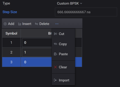
The figure below shows the four BPSK state changes described in the form above. The parameter, defined as 1/symbol rate, indicates the time duration at each phase state and determines the number of index items occurring during the 800 us pulse width time period for the New Pulse 1 pulse. For trapezoidal and raised-cosine pulse types the modulation is applied only during the duration of the pulse (Width (100%-100%)). For custom profile and custom IQ pulses the modulation is applied from the first point of data through to the last point of data.
Each state is offset 90 degrees from adjacent states. Step size is the time duration for each I/Q state (defined as 1/symbol rate).
The following figure shows QPSK phase state changes for a trapezoidal or raised-cosine pulse (Width (100%-100%)).
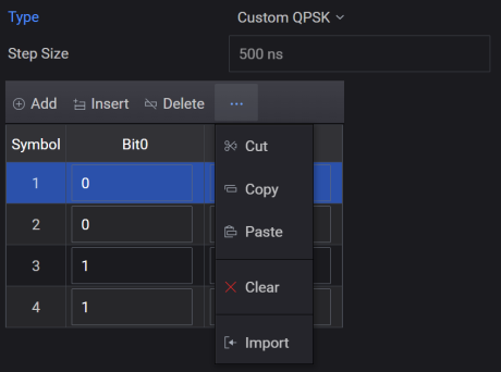
This table is used for the QPSK bit pattern. The symbol period is the pulse width (100%-100%) divided by the number of symbols. QPSK has two bits per symbol. The symbol mapping is as follows:
00 = 0°
01 = 90°
11 = 180°
10 = 270°
To add steps (index items) to the table:
Select Custom QPSK from the Modulation Type drop-down list box.
Click Add or Insert option to manually configure items in the Custom QPSK table or import from a csv file.
The Pulse Building application supports a number of Barker codes . When this modulation is selected, a drop-down list box, labeled Code Length is available in the GUI and displays the available Barker Codes.
Barker codes are binary numbers using two to 13 bits and have unique auto-correlation functions. The points adjacent to the peak of the correlation function equal zero. This is very useful in a radar system since any spurious response can be misinterpreted as a target. A Barker-coded pulse typically uses binary phase modulation.
The 'chip' rate is the dwell time for each bit within the pulse. A 7-bit Barker code contains the bits [+1 +1 +1 -1 -1 +1 -1]. The following table shows Barker Codes supported by the Pulse Building application.
|
Barker Code 2 |
10 |
|
Barker Code 3 |
110 |
|
Barker Code 4 |
1101 |
|
Barker Code 5 |
11101 |
|
Barker Code 7 |
1110010 |
|
Barker Code 11 |
11100010010 |
|
Barker Code 13 |
1111100110101 |
The figure below represents a 7-digit Barker code
The On and Off levels in this diagram correspond to a 180 degree phase shift (BPSK) in the carrier frequency.
The carrier is frequency modulated based on the user-defined Chirp Deviation parameter.
is the maximum change in the modulation frequency that occurs over the time period of the pulse (Width (100%-100%)) parameter for trapezoidal and raised-cosine pulse types and from the first point of data through the last point of data for custom profile and custom I/Q pulse types. The deviation is a ± value around the carrier frequency, so the actual frequency deviation is twice that indicated in the Chirp Deviation text box.
is calculated and displayed as a read-only reference value. Chirp rate for a trapezoidal and raised-cosine pulse type is calculated as: Chirp Rate = Chirp Deviation / pulse width. The maximum Chirp Rate is 80 MHz/uSec: 80 MHz/uSec > Chirp Deviation / pulse width.
For example, a pulse width of 0.1 uSec and a Chirp Deviation of 4 MHz has a Chirp Rate of 80 MHz/uSec. (2x4MHz)/0.1 uSec.
can be ascending or descending and indicates an increase or decrease in frequency during the FM chirp.
is held constant during pulse rise and fall times and is applied only during the duration of the pulse (Width (100%-100%)). In the form above the Chirp Deviation is ±40 MHz. During the pulse rise time the chirp frequency is 40 MHz below the carrier frequency. During the pulse width (100%-100%) the chirp frequency increases from 40 MHz below the carrier to 40 MHz above the carrier. During the fall time the chirp frequency is held at 40 MHz above the carrier.
The following figure shows the FM chirp deviation for the settings show above in the Pulse Details form.
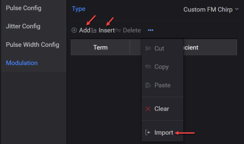
This mode allows you to define the Custom FM Chirp (non-linear) modulation within the pulse. The custom FM chirp is generated using a polynomial. This polynomial represents the instantaneous frequency versus time. The polynomial coefficients are entered into the Custom FM Chirp table by using the Add or Insert options or by importing the values from a .csv file. See Custom FM Chirp Example for more information.
Step size (time duration at each frequency step) and frequency offset from the carrier are user-defined. The frequency offset must be within the ±40 MHz bandwidth of the signal generator if using the internal Arb, or ±500 MHz if using the N603xA/M933xA or N824xA Arb. Selecting the FM Step Modulation Type displays a table as shown in the figure below.
For the trapezoidal and raised-cosine built-in pulse types the step size should sum to equal the pulse Width (100%-100%). For custom profile and custom I/Q pulse types the step size should sum to equal the time duration from the first point of data through to the last point of data. If the step size does not equal the pulse width the FM steps will be padded (if not enough steps), or truncated (if too many steps). Refer to the padded and truncated diagram for more information.
To create the FM Step table:
Select FM Step from the Modulation Type drop-down list box.
Configure items in the FM Step table or import from a csv file.
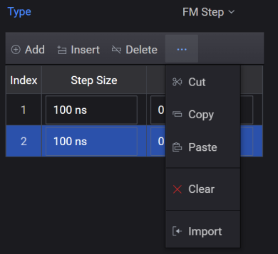
The following diagram shows the frequency offset and time duration relationship for the table entries in the form shown above.
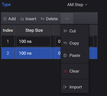
Step size in time and the amplitude of the carrier during the duration of the pulse are user-defined. Note that AM step is an intra-pulse modulation and not amplitude modulation from pulse to pulse. The amplitude offset is a relative parameter and must be within the power limits of the signal generator's baseband generator. The maximum amplitude is used as the reference; all lower power levels are relative to the maximum amplitude step.
For the trapezoidal and raised-cosine built-in pulse types the step size should sum to equal the pulse Width (100%-100%). For custom profile and custom I/Q pulse types the step size should sum to equal the time duration from the first point of data through to the last point of data. Selecting the AM Step Modulation Type displays an AM step table shown in the figure below. If the step size does not equal the pulse width, the AM steps will be padded (if not enough steps), or truncated (if too many steps). Refer to the padded and truncated diagram for more information.
When using the AM Step modulation format, the ALC should be turned off using the Keysight PathWave Signal Generator software. This prevents the ALC from trying to level the AM step within the pulse.
To create the AM step table:
Select AM Step from the Modulation Type drop-down list box.
Configure items in the AM Step table or import from a csv file.
In the following diagram, the frequency offset and time duration relationship for the table entries in the above figure are shown. Note that modulation is applied only during the pulse Width (100%-100%) time interval and not during rise and fall times. In the diagram below the last half of the –15 dB step, and the entire 0 dB step will not modulate the pulse because they occur after the pulse width of 8 us. See the section on padding and truncating.
This is a polyphase code modulation format used for pulse compression.
The default Frank code Code Order is N = 4.
The Frank Code has N2 elements and is defined as:
i,j
Where i and j range from 1 to N. For example, the Frank Code with N = 4, by taking phase value modulo is given by the following sequence:
0
0
0
0
4x4
0
0
0
0
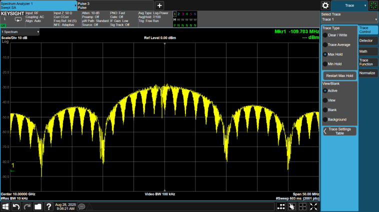
The figure below shows the spectrum of a 10 us pulse using Frank Coded phase modulation, where N = 10.
The P1 code is a modified version of the Frank code where the DC frequency term is in the middle of the pulse instead of at the beginning.
The default P1 code Code Order is N = 4.
The P1 code has N2 elements and is defined as:
i,j
Where i and j range from 1 to N. For example, the P1 code with N = 4, by taking phase value modulo is given by the following sequence:
0
0
4x4
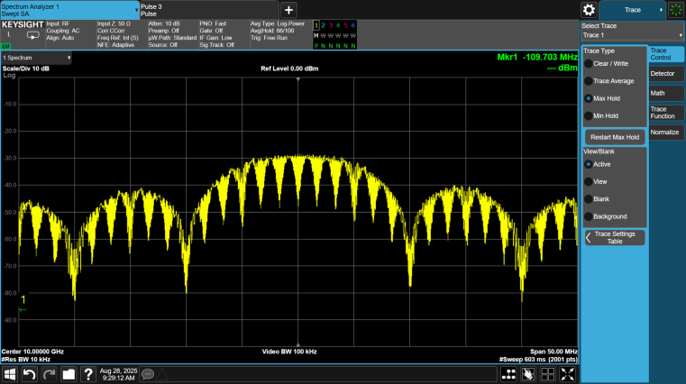
The figure below shows the spectrum of a 10 us pulse using P1 Coded phase modulation, where N = 10.
The P2 code is a modified version of the Frank code where the DC frequency term is in the middle of the pulse instead of at the beginning. The P2 code is only valid for even code orders (N = 2, 4, 6, 8...)
The default P2 code Code Order is N = 4.
The P2 code has N2 elements and is defined as:
i,j
Where i and j range from 1 to N. For example, the P2 code with N = 4, by taking phase value modulo is given by the following sequence:
4x4
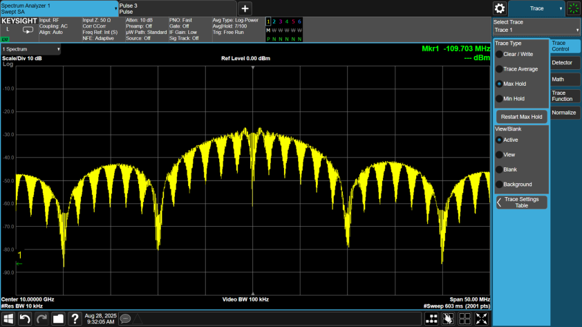
The figure below shows the spectrum of a 10 us pulse using P2 Coded phase modulation, where N = 10.

The P3 code does not require a square matrix like the Frank, P1, and P2 codes. The code order (N) is the number of values in the phase pattern. The number of items in the Frank, P1, and P2 codes patterns is N2.
The default P3 code Code Order is N = 16.
The P3 code has N elements and is defined as:
i 2
Where i ranges from 1 to N. For example, the P3 code with N = 16, by taking phase value modulo is given by the following sequence:
16
=
0
0
The figure below shows the spectrum of a 10 us pulse using P3 Coded phase modulation, where N = 100.
The P4 code does not require a square matrix like the Frank, P1, and P2 codes. The code order (N) is the number of values in the phase pattern. The number of items in the Frank, P1, and P2 codes patterns is N2
The default P4 code Code Order is N = 16.
The P4 code has N elements and is defined as:
i
Where i ranges from 1 to N. For example, the P4 code with N = 16, by taking phase value modulo is given by the following sequence:
16
=
0
0
The figure below shows the spectrum of a 10 us pulse using P4 Coded phase modulation, where N = 100.

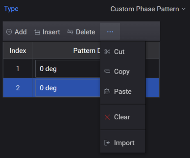
The custom phase code modulation applies a user-provided phase pattern to the pulse. The user phase code is entered into a table and is assumed to be in degrees. Complex polyphase patterns can be generated with MatLab or other tools.
To add steps (index items) to the table:
Select Custom Phase Pattern from the Modulation Type drop-down list box.
Configure items in the Custom Phase Pattern table or import from a csv file.
Following is a simple example using the custom phase code modulation to generate a Barker 13 phase coded signal.