Pulse Measurement Basics

When making Pulse measurements, the VSA software allows individual acquisitions long enough to contain multiple pulses.

The signal being analyzed may come from an external down converter, in which case the VSA Software’s external down converter feature can be used to ensure that traces and results have correct frequency labeling.

Segmented Capture

The VSA software also allows you to use “segmented capture”, which is helpful when using measurement hardware such as an oscilloscope. When using segmented capture in a live measurement, you set the Segment Length parameter to specify the length of a single segment, and then separately specify the number of segments to use in the measurement. The measurement therefore contains an integer number of segments from the hardware. Each segment starts at a trigger point as defined by the input trigger settings.

You can record and play segmented captures. Recording size is not limited by the acquisition limit. When playing a recording that contains segmented data, Pulse measurements work the same as a live measurement and allow multiple segments to be within each time record obtained from the recording.

If the recording contains segmented data, the VSA software constrains your settings for acquisition length to fit within a single segment, and then separately allows the number of segments to be specified – just like a live measurement. If your time/RBW Resolution Band Width (RBW or ResBW): specifies the minimum frequency bandwith that two separate frequency spectra can be resolved and viewed seperately. For FFT (digital) based VSA's the process is equivalent to passing a time-domain signal through a bank of bandpass filters, whose center frequencies correspond to the frequencies of the FFT bins. For a traditional swept-tuned (non-digital) spectrum analyzer, the resolution bandwidth is the bandwidth of the IF filter which determines the selectivity. settings require a shorter time length than the recording segment length, the measurement receives that amount of time data from the start of each segment in the recording. This ensures the playback measurement does not get unexpected results due to discontinuities or incorrect start/stop times.

See Segmented Data Acquisition for more information.

Pulse Assumptions

The Pulse Measurement Software makes the following assumptions about the nature of RF Radio Frequency: A generic term for radio-based technologies, operating between the Low Frequency range (30k Hz) and the Extra High Frequency range (300 GHz). pulses to be measured, and uses the algorithms and analysis approaches described below. Where possible, the methods used conform to IEEE Institute of Electrical and Electronics Engineers. A US-based membership organisation that includes engineers, scientists, and students in electronics and related fields. The IEEE developed the 802 series wired and wireless LAN standards. Visit the IEEE at http://www.ieee.org Std 181 – 1977 “Standard on Transitions, Pulses, and Related Waveforms.” In addition, certain approaches are based on generally accepted procedures for the industry, and/or to maintain consistency with other measuring equipment.

A typical pulse is assumed to have a format as follows:

The pulsed signal is concentrated into two clearly-separated states: On and Off.
The transitions from Off to On, or On to Off, are relatively short compared to the duration of On and Off intervals.
Each pulse “cycle” begins with a transition from Off to On; continues On for a period that is free of large amplitude variations; then transitions from On to Off; and continues Off for a period that is continuously without signal present. The minimum On period is specified for each instrument (depends on highest sample rate). The Off-to-On and On-to-Off transitions can be arbitrarily short, but the system’s ability to actually represent the signal or measure what this time is will be limited for each instrument.
If there is a large amplitude “drop out” (dip) during the On interval, or a signal “spike” in the Off interval, the software may misrepresent these as separate pulse cycles. Note that you can use the ignore dropouts feature to ignore drop outs or spikes.

You can typically adjust Acquisition Length to capture only a portion of a single pulse cycle, or capture many pulse cycles. The Pulse Measurement software will analyze as many parameters as possible, for as many pulses as possible, but an incomplete pulse cycle will be ignored.

Pulse Detection

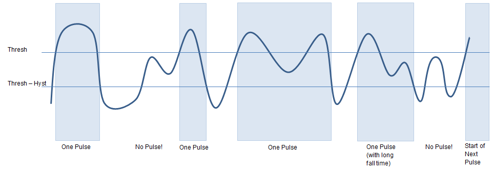
A pulsed signal is a signal whose carrier power is modulated between an ON and OFF state. A pulse is detected when the input signal power exceeds a threshold, then subsequently falls below that threshold, or vice versa. Pulses that rise to and remain at a peak (positive) power level for a certain duration, and then fall again are positive pulses. A negative transition is the opposite-- it falls and remains at a minimum (negative) power level, and then rises. The "ON" power level is referred to as the top or 100% level. The "OFF" level is referred to as the base or 0% level.

A hysteresis allows you to modify the detection process and avoid falsely interpreting unstable signals as pulses. Detection can also be restricted to a maximum number of pulses. The illustration below shows valid pulses when both a threshold and hysteresis are specified.

Pulse Computations

The basic computation for Pulse measurements consists of:

Synchronizing the measured data with reference data.

Synchronization consists of time-aligning the measured and reference data (using cross-correlation). Synchronization normalizes the measured data so that the reference has an RMS level of 1.

The measured data may contain multiple pulses. After time alignment, amplitude alignment is performed between the measured and reference data, because each pulse amplitude may vary.
Some of the computed metrics depend on thresholds for pulse width, rise time, etc. By default, the VSA Software uses values as specified in IEEE 181-2011 (for example, rise time goes from 10% to 90%). However, you can manually change the thresholds. When computing values for each pulse,you can exclude the beginning and end of the pulse/region from affecting the calculations. For example, you may want to exclude the first and last 10% of each region in an FMCW Radar analysis. In addition, you may want to exclude a different amount during synchronization than is excluded during the analysis calculations--the VSA software provides separate settings for the synchronization and analysis calculations. When you define the exclusion zone, you can specify a percent of region length, or an absolute time in seconds. You can also control the aperture used when computing frequency and phase-related values. This aperture is separate from the aperture used by the VSA software when displaying group delay.
For each scalar result, you can view average, max, rms, min, and standard deviation across multiple pulses and multiple measurements. You can also view a trend line or histogram that spans multiple pulses/regions and multiple measurements. You can remove the mean, slope, and/or second-order term before displaying the trend line or histogram. The trend and histogram traces for all scalar results are available as separate trace types, so that the trend lines for several different scalar values can be displayed at the same time, and possibly overlaid on the display.

You can specify a “stop measurement” condition by specifying a scalar result, along with a threshold and the comparison operator (equal, not equal, less than, greater than, less than or equal, greater than or equal). If the measurement is a continuously running measurement and the stop condition is met, the measurement is stopped.

Two-Channel Pulse Difference Analysis

The Pulse Measurement Software supports difference analysis when the hardware configuration contains two or more channels. With difference analysis, the pulse measurement uses channel 1 as the “reference." Like single-channel pulse measurements, all pulse measurement results are available for the reference channel.

Channel 2 is expected to be similar to channel 1, but channel 2 pulses may have different timing, amplitude, and frequency than the corresponding channel 1 pulses. Channel 2 has a subset of the channel 1 results (see Available Trace Data). Additionally, three new columns are added to the Pulse Table for pulse difference analysis: Ch2 Time Difference (in seconds), Ch2 Amplitude Difference (in dB), and Ch2 Frequency Difference (in Hz). There are also three new Trend Line Traces and three new Histogram Traces, one for each of the new columns in the Pulse Table.