The following features can be used after a measurement to analyze the results.
In this Chapters
“Auto Sync Limit (EMF scan mode Limit Lines Only)” on page 840 |
“Averaging (CAT, NA, Power Meter, Channel Scanner, and Pulse Measurement Modes Only)” on page 853 |
Markers move along the X-axis range of the measurement trace to provide a numerical readout of each measured data point. Markers also allow you to search for specific Y-axis values.
A trace can contain up to six markers.
The marker readout on the FieldFox screen displays X and Y-axis information for the current active marker ONLY.
A Marker Table can be displayed that allows you to simultaneously view X and Y-axis information for all markers.
Markers can be used in CAT, EMI Measurements, I/Q Analyzer, NA, NF, RTSA, SA, Phased Array Antenna, and Pulse Measurements Modes.
1.Press Marker.
2.Then Markers 1...6 to select a marker to activate.
3.Then Normal to activate that marker. A marker is created on the trace in the middle of the X-axis. That marker is now active.
4.Then move the marker using the rotary knob, the  arrows, or by entering an X-axis position with the number keys.
5.Then press Enter.
How to move a Marker after it is created
—Press Marker.
—Then Markers 1...6 repeatedly until the marker of interest is selected. The OFF, Normal, or Delta softkey is black to indicate the current setting of each marker.
—Then move the marker as when it was first created.
—Markers can also be moved using one of the marker search functions. Refer to “Searching with Markers” on page 825.
Figure 30-1 Marker 2 is Active, marker 1 is NOT active.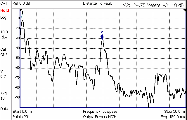
A Delta marker provides X-and Y-axis readout information that is relative to a ‘reference’ marker.
A Delta marker is created with a D (delta symbol) to distinguish it from the reference marker.
All six markers can be a Delta marker pair.
Peak search functions can be performed using delta markers.
Figure 30-2 A Delta marker and its associated reference marker. 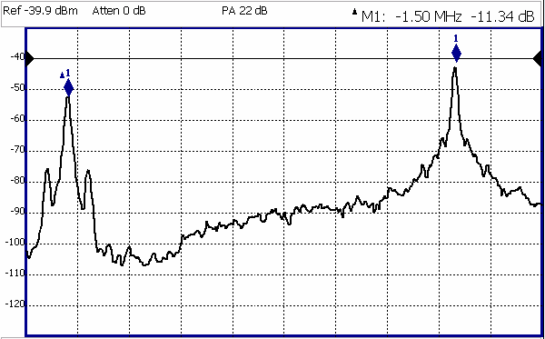
In the graphic above, the marker readout shows the difference between the two markers in frequency and amplitude.
—Create a Normal marker and move it to the reference position.
—Press Delta. The marker becomes the reference marker and fixed in its X-Axis position.
—Move the Delta marker using the numeric keypad, the arrows, or the rotary knob.
—Press Enter when finished.
How to move the Reference marker
—Press Normal to turn the Delta marker OFF.
—Move the marker to the new position.
—Then press Delta again, to turn the Delta marker back ON.
Fix the position of the Reference marker (I/Q Analyzer, RTSA, and SA Modes ONLY)
In SA mode, the reference marker can be fixed at the Y-axis position of the data trace when the marker was created, or it can ‘float’ with each sweep at the Y-axis position of the data trace. In CAT and NA mode, the reference marker always floats with the data trace.
—Create a Delta marker.
—From the Mkr ->/Tools menu, press More (SA mode only), then Marker Properties, then Delta Ref Fixed
—OFF – The reference marker floats at the data trace Y-axis position.
—ON – The reference marker is fixed at the Y-axis position of the data trace when the marker was created (Default IQA and SA modes).
Signal Track Marker (NF and SA Mode ONLY)
In NF and SA mode, the marker can be peaked at the Y-axis position of the data trace and the marker is centered on the screen. This setting applies to all NF and SA markers.
—Create a Signal Track marker (peak).
—From the Mkr ->/Tools menu, press More, then Marker Search
—OFF – The reference marker floats at the data trace Y-axis position.
—ON – The reference marker is peaked at the Y-axis position of the data trace and the marker is centered on the screen.
The Marker Table can be displayed at the bottom of the FieldFox screen. It can display information for up to 6 markers in a full-width window, and up to 3 markers for a half-width window (NA mode). The marker table “squeezes” the graticule area when activated.
How to display the Marker table
1.Press Marker.
2.Then More
3.Then Marker Table On Off.
| I/Q Analyzer (IQA) mode has coupled markers. but the behavior is different than the NA mode Coupled Markers behavior. Refer to “Coupled Markers (Waveform Only)” on page 336. |
Coupled Markers, available in NA mode only1 and allows you to simultaneously create and move markers that have the same number for all traces. For example, when marker 2 is created on a trace, a marker 2 is created for ALL traces. When any marker 2 is moved, they all move together to the same X-axis position.
—Coupled markers are allowed only in NA mode and are relevant only in multi-trace configurations.
—You can have markers that are coupled and others that are uncoupled.
—Peak functions move the marker to the peak on the active trace, while all other markers move to the same X-axis position.
Figure 30-3 Coupled Markers move on ALL traces at the same time (NA shown).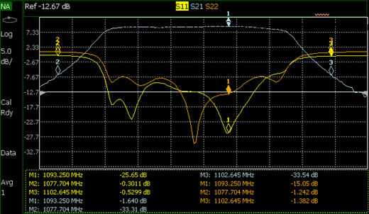
How to create Uncoupled Markers
| Markers are coupled by default. |
To create markers that are NOT coupled (move independently on each trace):
1.Press Marker
2.Then More
3.Then Coupled Markers OFF
As shown in the above image, in NA and CAT Modes, markers are the same color as the trace to which they are assigned. In SA Mode, the marker color is NOT the same as the trace.
Marker colors can NOT be changed.
Marker Trace (CAT, NA, NF Modes)
The Marker Trace setting is used to move markers between the data trace and memory trace.
When Coupled Markers is ON, this setting applies to the active marker for ALL traces that are coupled. Otherwise, this setting applies to the active marker on only the active trace.
How to move a CAT, NA, and NF mode marker between traces
1.With at least one marker present, press Marker then More.
2.Then select the marker to move using Marker 1,2,3,4,5,6.
3.Then toggle Marker Trace Auto Data Mem.
—Auto - Marker resides on data trace when it is visible. Marker resides on memory trace when only IT is visible (Default setting).
—Data - Marker resides on data trace, even when not visible.
—Mem - Marker resides on memory trace, even when not visible.
Marker Trace (IQA and SA Mode)
Marker Trace determines the trace number on which a marker resides. A marker is created on, or can later be changed to, the trace number specified by the Marker Trace selection. When changed, a marker moves to the same X-axis location on the specified trace.
Learn more about IQA Traces in “Trace Display States (IQA Mode)” on page 339.
Learn more about SA Traces in “Trace Display States (SA mode)” on page 213.
How to move an IQ and SA mode marker between traces
1.With two or more traces present, press Marker and Enter to create a marker. The marker is created on the current Marker Trace selection (Default == 1).
2.Then More
3.Then select the marker to move using Marker 1,2,3,4,5,6.
4.Then toggle Marker Trace 1,2,3,4
—The selected marker is moved to the specified trace.
—When a marker is moved to a ‘blank’ trace (not visible) the marker moves to the same X-axis position at either the Y-axis position of the last data, or to the ZERO position.
The Marker Format setting allows you to choose the format of the marker readout that appears in the upper-right corner of the screen and in the marker table. The marker format can be independent of the trace format, and can be set independently for each trace. All markers on a trace have the same marker format.
How to choose marker format
—Press Marker
—Then More
—Then Marker Format
—For NA Mode measurements, choose from the following:
Selection | Example Y-axis value |
|---|---|
Default Same as displayed format | |
R + jX Complex impedance format | 22.8Ω -j61.4Ω 287.9fF |
Z Magnitude Impedance Mag. | 66.08Ω |
Phase | 73.8° |
Real | 0.2003 |
More | |
Imaginary | -0.6727 |
Mag & Phase | 0.705, -73.7° |
dB Angle | -2.1 dB, -138.2° |
There are more trace formats available than marker formats. To display marker readouts in more formats than are shown here, change the trace format, then select Default. Learn how to change format in “Format” on page 104.
—For TDR (CAT) Mode, choose from Default and Z Mag.
Marker Searches are used to move markers to locations on the trace which exhibits the characteristics of the search criteria. Learn What is a ’Peak’ in “What Is a ‘Peak’” on page 830.
The following menu structure applies to NA Mode. Keystrokes will be slightly different for CAT, Pulse Measurements, and SA Modes.
1.Activate the marker to be used for the search (NOT necessary with Bandwidth search.)
2.Then press Mkr ->/Tools.
3.Then choose one of the following:
—Tracking ON OFF (NA Mode ONLY)
—ON causes the active marker to search for the specified criteria with each new sweep. Search criteria can include: Target, Bandwidth, Peak, Min. The searches begin with the first sweep after Tracking is turned ON, based on the current search type. Trk appears next to the marker number.
—OFF causes a new marker search only when the search feature is re-executed.
—Peak Moves the active marker to the HIGHEST amplitude data point of the trace. Peak Excursion and Peak Threshold value is ignored. In SA Mode, the LO feed-through signal (0 Hz) is also ignored.
—Next Peak Moves the active marker to the next highest amplitude data point of the trace. Peak Excursion value is ignored.
—Mkr -> Center Moves the current active selected marker to the center frequency for the current frequency range displayed.
—Mkr -> RefLev Moves the current active marker to the acquisition.
—Minimum (Not available in DTF, RTSA, SA, or I/Q Analyzer) Moves the active marker to the LOWEST amplitude data point of the trace.
—Min Search (I/Q Analyzer, RTSA, and SA modes Only) Moves the active marker to the LOWEST amplitude data point of the trace. If a marker is turned off, it is turned on before the minimum search is performed.
—Target (NA Mode and Pulse Measurements ONLY) Enter the Target value. The marker moves to the first occurrence of the Target value to the right of its current position. The FieldFox interpolates between measured data points to find the exact Target value to two decimal points. The interpolated X-axis value is displayed in the marker readout or marker table. Subsequent presses of the Target softkey cause the marker to move to the right to find the next occurrence of the Target value. When the marker reaches the end of the stimulus range, it “wraps around” and continues the search from the beginning of the stimulus range.
—Bandwidth ON OFF (NA Mode ONLY) Use to quickly toggle BW Markers ON and OFF. When OFF, the marker table appears showing the X and Y-axis positions of all enabled markers.
—Bandwidth (NA Mode ONLY) Specify the level in dB from the peak or valley where bandwidth is measured.
—Negative numbers search for a Peak bandpass, such as a filter S21 response.
—Either of the following TWO methods can be used to search for a Valley or Notch filter, such as the S11 response of a bandpass filter.
—Negative values search down from the TOP (MAX) of the response.
—Positive values search up from the BOTTOM (MIN) of the notch.
—If you first enter Negative, then Positive values, it may be necessary to press Marker, then More, then Markers All Off.
Figure 30-4 S21 of a filter with BW Markers and associated readout values. The search criteria is -3 dB.
Figure 30-5 S11 of the same filter with same search criteria: -3 dB.
The same values would result from a search criteria of approximately +30.4 dB.
After pressing Bandwidth, four markers are automatically created to find the first negative or positive bandpass over the displayed frequency range.
Bandwidth Search can be used ONLY with Log Mag display format.
—The following six values are displayed for Bandwidth Search:
—BW: Width of the filter. (marker 2 freq) minus (marker 3 freq).
—Center: Marker 4 frequency. Mathematical midpoint between marker 2 and marker 3.
—Q: Center Frequency / Bandwidth.
—Loss: Marker 1 amplitude.
—Left: Frequency of marker 2 or 3 (to left of marker 1).
—Right: Frequency of marker 2 or 3 (to right of marker 1).
—Press Back to return to the previous menu.
Press Peak Search then choose from the following:
—Peak Moves the active marker to the HIGHEST amplitude data point of the trace. Peak Excursion value is ignored. In SA Mode, the LO feed-through signal (0 Hz) is also ignored.
—Next Peak Moves the active marker to the next highest amplitude peak from where it currently resides.
—Peak Left (Not IQA) Moves the active marker to the next data point to the left that meets the ‘Peak’ criteria. When no data points to the left meet the ‘Peak’ criteria, the marker does not move.
—Peak Right (Not IQA) Moves the active marker to the next data point to the right that meets the ‘Peak’ criteria. When no data points to the right meet the ‘Peak’ criteria, the marker does not move.
The following applies to DTF Measurements ONLY:
—Track Peaks ON OFF When Track Peaks is ON, markers will find the new peak with every sweep. While in this Mode, the markers can NOT be turned OFF or moved.
—Find 3 Peaks Three markers are created and find the highest peaks (faults) on the trace.
The following applies to IQA Measurements ONLY:
—More then:
—Min Search Moves the active marker to the minimum frequency (IQA displays time) currently displayed on the screen.
—Mkr Properties then:
—Peak Criteria then refer to “How to set Peak Criteria” on page 830:
—Delta Ref Fixed Enables or disables the delta reference fixed marker.
—Peak Left (IQA Spectrum Only) Moves the active marker to the next data point to the left that meets the ‘Peak’ criteria. When no data points to the left meet the ‘Peak’ criteria, the marker does not move.
—Peak Right (IQA Spectrum Only) Moves the active marker to the next data point to the right that meets the ‘Peak’ criteria. When no data points to the right meet the ‘Peak’ criteria, the marker does not move.
Using Mkr5/Mkr6 to find mins/maxs between Mkr1 and Mkr2 / Mkr3 and Mkr4 (CAT and NA Mode)
Use this feature to search minimum and maximum values within sub-spans defined by Mkr1 and Mkr2, and Mkr3 and Mkr4. This facilitates measuring minimum and maximum values on your uplink and downlink channels, or only in the passband of a DUT. Use in conjunction with marker table and limit lines to verify your DUT’s signals and to adjust or tune as needed. See also, “All about Limit Lines” on page 834.
When markers are set to Normal, Mkr5 and Mkr6 can be used to find the minimum and or maximum values between Mkr1 and Mkr2 (using Mkr5) and Mkr3 and Mkr4 (using Mkr6). Refer to Figure 30-6 on page 830.
| If your Markers are positioned and in Normal marker mode, no changes are made to the Mkr1 through Mkr4 settings. —Markers are all set to Normal —Mkr1 and Mkr3 are set to 1/4 full span —Mkr2 and Mkr4 are set to 3/4 full span |
How to use the Mkr5 and Mkr6 markers to find maximums and minimums between your Normal markers (CAT and NA Mode):
This section assumes you understand the previous marker features. And, that you have previously positioned your markers (Mkr1 and Mkr2 or and Mkr3 and Mk4) and set the markers up as Normal markers using “How to create Markers” on page 819 and other previous marker sections. For example, if your markers are set to Delta, change to Normal, and verify the marker positions are correct. Refer to Figure 30-6 on page 830.
—Then press Mkr ->/Tools.
—Then More (For DTF, TDR measurements, and NA Mode, skip this step and proceed to the next step.)
—Then Mkr5 & Mkr6 Search
—For Mkr1 & Mkr2 maximum or minimum value search:
—Then Mkr5 Peak or
—Mkr5 Min
Or for Mkr3 & Mkr4 maximum or minimum value search:
—Then Mkr6 Peak or
—Mkr6 Min
Figure 30-6 CAT Mode Mkr5 and Mkr6 Search Example
You define what the FieldFox considers a “peak” by setting the Peak Threshold and Peak Excursion and for I/Q Analyzer Only Cont Peak Search.
These two peak criteria settings are set individually for each trace and for each mode (CAT, SA, or NA).
These settings do NOT survive a FieldFox or Mode Preset.
| The Peak Threshold and Excursion settings are NOT available in DTF measurements. To make these settings, create a non-DTF CAT mode measurement, then change the measurement back to DTF. |
—Press Mkr ->/Tools.
—In CAT and NA modes:
—Then Peak Search.
—Then Peak Criteria
—In IQA (Spectrum) and SA mode:
—Then More
——Then Mkr Properties
——Then Peak Criteria
—In IQA (Waveform) mode:
—Then Mkr Properties
——Then Peak Criteria
After selecting Peak Criteria for CAT, IQA, NA, or SA mode:
——Then select the following:
——Peak Threshold Minimum amplitude (dB). To be considered valid, the peak must be above the threshold level. The valley on either side can be below the threshold level.
Default == –190 for CAT and NA Modes; –90 for SA Mode.
| CAT mode Loss measurements are displayed in positive values. In these cases, the Peak Threshold setting is inverted. For example, Peak Threshold = –20 will consider any peak that has less Loss than 20 dB to be valid. |
——Peak Excursion The vertical distance (dB) between the peak and the valleys on both sides. To be considered a peak, data values must “fall off” from the peak on both sides by the excursion value. Default == 0.5 dB for CAT and NA Modes; 6 dB for SA Mode.
——Cont Peak Search (I/Q Analyzer Only) Enables or disables the Continuous Peak Search marker. When Continuous Peak Search is on, a peak search is automatically performed for the selected marker after each sweep. The rules for finding the peak are exactly the same as for Peak Search, including the use of peak criteria rules. See also, “Using Markers (IQA)” on page 334.
——Delta Ref Fixed Enables or disables the delta reference fixed marker.
Peak Excursion and Peak Threshold example—the settings for the trace in the following image are:
——Threshold: –10 dB
——Excursion: 1 dB
——Scale = 1 dB / Division.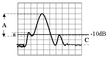
Peak A = Valid Peak (Above Threshold and Excursion Settings)
Peak B = Invalid Peak (Below 1 dB Excursion Setting)
Peak C = Invalid Peak (Below –10 dB Threshold Setting)
Marker functions are used to change FieldFox frequency or distance settings to those of the active marker.
1.Activate the marker to move.
2.Then press Mkr ->/Tools
3.Then Mkr -> (this step not required for all modes)
4.Then choose one of the following:
—Mkr -> Center (Not available in DTF, I/Q Analyzer (waveform), or SA mode with zero span) The center frequency of the measurement becomes the value of the active marker. The frequency span is adjusted accordingly.
—Mkr -> Delay (NA mode ONLY.) The group delay value of the active marker becomes the electrical delay setting of the trace. Learn how to set group delay format in “Calibration Settings” on page 103. Learn more about electrical delay in “Electrical Delay” on page 107.
—Mkr-> RefLev (IQ Analyzer (NOT waveform) and SA mode ONLY) The acquisition becomes the magnitude of the active marker.
—Mkr->TuneFreq (SA mode with Tune & Listen ONLY) The Tune & Listen Frequency becomes the frequency of the active marker (When AM Metrics or FM Metrics are selected this softkey is inactive).
The following applies to DTF Measurements ONLY:
—More then:
—Mkr->Start Distance The Start Distance of the measurement becomes the value of the active marker. Markers that would no longer appear on the screen are moved to the new Start Distance.
—Mkr->Stop Distance The Stop Distance of the measurement becomes the value of the active marker. Markers that would no longer appear on the screen are moved to the new Stop Distance.
I/Q Analyzer (IQA) Marker Functions
The following Marker Functions are available in I/Q Analyzer Mode ONLY (exceptions are noted):
—Noise Marker (Available in SA mode)
—Band/Interval Power Marker (Available in SA mode)
—Coupled Markers
—Continuous Peak Search
Learn more about Noise and Band/Interval Power marker functions starting in the IQA chapter here: “Noise Marker” on page 334.
The following Marker Functions are available in SA Mode ONLY (exceptions are noted):
—Noise Marker (Available in I/Q Analyzer mode)
—Band/Interval Power Marker (Available in I/Q Analyzer mode)
—Frequency Counter at Marker
—Audio Beep with Marker
Learn more about these marker functions starting in the SA chapter here: “Noise Marker” on page 227.
Limit lines are visual representations, drawn on the FieldFox screen, of the specified limits for a measurement. With this capability, you can easily compare measured data versus specifications. Optionally, you can enable an audible beep and display Pass or Fail information for each measurement. IMPORTANT! For CAT and NA modes, limit lines do not apply
where F1 = F2.
—You can have up to as many limit line segments as there are data points for each measurement trace allowing you to test all aspects of your measurements.
—Limit lines are available in CAT Mode, NA Mode, NF Mode, and SA Mode. Power Meter Mode uses different limit settings. Learn more in “Limits” on page 619.
—Limit lines and limit testing are NOT allowed in NA Mode with Smith Chart or Polar display formats.
—A simple Display Line is also available in I/Q Analyzer, NF, and SA Modes ONLY. Learn more in “Display Line (I/Q, NF, and SA Modes Only)” on page 849.
—Limit lines can be saved and recalled with an *.sta file. Learn more in“How to Save and Recall Limits” on page 840. *.sta files can also be saved and recalled independently from the Limit softkeys. Learn more inChapter 33, “File Management.”
How to Create Fixed Limit Lines
There are two ways to build a Fixed limit line:
1.Build (limits) From a Trace. Learn how in “Build From Trace” on page 837.
2.Enter X/Y data points into the on-screen editor. The limit line is formed as the FieldFox ‘connects the dots’ on the screen. To create frequency gaps that are NOT tested, use separate limit lines. The X-axis values for two lines can overlap.
3.Press Limit 8 > Edit Limits. A limit line table appears.
4.Use the Up / Down arrows and rotary knob to navigate the cursor to the following editable cells.
—Description - Press Edit, then enter a description for the limit line using the FieldFox labeler. Learn how in “How to use the FieldFox labeler ” on page 916.
—Fixed/Relative – Press Edit to toggle between the following:
—Fixed - (Default) the limit line does not move. The X/Y coordinates are absolute locations on the screen.
—Relative - the limit line moves relative to the center frequency and acquisition. Note: It is easiest to first create Fixed Limits, then change this setting to Relative. Learn more “Relative Limit Lines” on page 836.
—Upper/Lower – Press Edit to toggle between the following: In Channel Scanner EMF Custom List scan mode, —Only limits configured as “Upper” limit types will be utilized for testing and displayed graphically. —If the limit is configured as “Lower”, it will be ignored in this mode, regardless of the limit is configuration as “ON” or “OFF”.
—Upper:
——All modes except RTSA: (Default) FAILS any measured data point ABOVE the line.
——RTSA mode: (Default) Draws visible “ears” going upward from any measured data point BELOW the line.
—Lower:
——All modes except RTSA: FAILS any measured data point BELOW the line.
——RTSA mode: Draws visible “ears” going downward from any measured data point ABOVE the line.
—Off/On – Press Edit to toggle between the following:
—On:
——All modes except RTSA: Limit line is drawn on the screen and PASS/FAIL testing occurs.
——RTSA mode: Limit line is drawn on the screen, but no PASS/FAIL testing occurs.
—Off: -- All modes: Limit line is NOT drawn on the screen and testing does NOT occur.
—Frequency – Enter a numeric X-axis value of the data point.
—Amplitude – Enter a numeric Y-axis value of the data point.
5.Then optionally choose from the following:
—Press Add then choose from the following:
—Add Point - Adds a blank X/Y data point below the cursor.
—Add Limit - Adds a default limit line below the current limit.
—Press Clear then choose from the following:
—Clear Point - Removes the X/Y data point on which the cursor resides.
—Clear Limit - Removes the limit Line on which the cursor resides.
—Clear All - Removes ALL limit lines.
—Press <Back to return to the Limit menu.
Relative limit lines are X/Y coordinates that are referenced to the center frequency (X-axis) and acquisition (Y-axis).
Use relative limits to test devices or signals that are identical except for the center frequency or amplitude. With relative limit lines in place, you change the center frequency of the measurement and the limits look as though they are in the same location.
The same is true for acquisition. When you expect to measure a different power level, instead of changing the Y-axis value of all of the fixed limits, simply change to relative limits. The limits will then remain a constant Y-axis distance from the acquisition.
Each limit line can be changed at any time from Fixed to Relative, and Relative to Fixed.
How to Create a Relative Limit Line
The easiest way to create a Relative limit line is to create a Fixed Limit at a specific center frequency and acquisition. Learn how “Relative Limit Lines” on page 836. Then change the limit line to Relative. The X/Y data points will be re-calculated relative to the center frequency and acquisition.
A limit line can be built from an existing trace. One X/Y point is made from each measured data point. Then, using an offset value, you can shift the limit line UP for upper limits or DOWN for lower limits.
Once limit lines have been built from the trace, changes that you make to the trace, such as frequency range, do NOT change the limits. However, the limit line properties can be edited just like standard limit lines.
Figure 30-7 A lower limit line (red) built from the trace (yellow) shifted down 5 dB.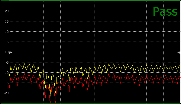
How to Build Limit Lines from a Trace
| Build from Trace is NOT allowed for traces with more than 1001 data points. |
1.Select the trace from which limits will be built.
2.Press Limit 8 > Edit > Build From Trace. A limit line table appears.
Figure 30-8 Build From Trace (1 of 2)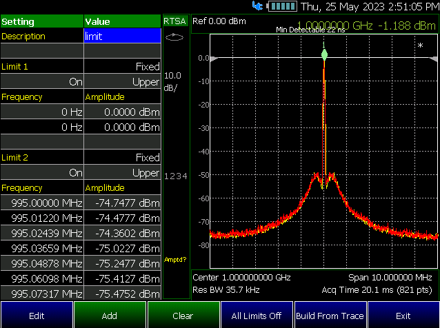
3.Use the arrows to select ON.
4.Use Offset to shift the limit line UP or DOWN. Learn how below.
Figure 30-9 Build From Trace (2 of 2)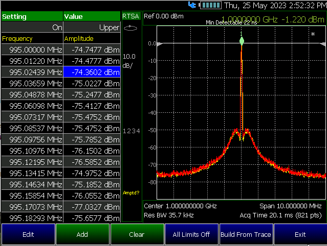
How to set Limit Options
1.Press Exit if the limit table is visible.
2.Then Options.
3.Then choose from the following:
—Beep
—On Pass Audible beep sounds when a sweep passes.
—On Fail Audible beep sounds when a sweep fails.
—Warning On Off Shows Pass or Fail indication on the display with each sweep. Data points that fail are highlighted.
—Limit Type Then Fixed or Relative.
—Offset Only available when the units are in V/m in SA mode.
—Offset Type dB % Press to toggle Offset Type from dB to %. (Default == dB).
—dB Offset 0.0 dB Adjust the limit line up or down by dB offset when toggle Offset Type to dB.
Enter desired offset value using the rotary knob, the arrows, or by entering a value with the number keys.
—% Offset 100.0% Adjust the limit line up or down by % offset when toggle Offset Type to %.
Enter desired % offset value using the rotary knob, the arrows, or by entering a value with the number keys.
Offset Available only when the units are not in V/m in SA mode. Shifts the limit line up or down. Enter an offset value using the rotary knob, the arrows, or by entering a value with the number keys.
—Enter a positive offset to shift the limit line UP, usually used with UPPER limits.
—Enter a negative offset to shift the limit line DOWN, usually used with LOWER limits.
—Margin Shifts the limit line up or down like an offset, but only virtually. The limit line does NOT appear to move. Enter a Margin value using the rotary knob, the arrows, or by entering a value with the number keys.
Enter a positive margin to virtually shift the limit line UP.
Enter a negative margin to virtually shift the limit line DOWN.
—LogX Interp Auto Off Enables/disables the logarithmic X-axis interpolation trace (Default == Auto). Learn more, refer to “Logarithmic X-axis Interpolation (EMI and SA modes Only)” on page 229.
Auto Sync Limit (EMF scan mode Limit Lines Only)
By enabling or disabling this Auto Sync Limit feature, users can control whether the limits set in the limit line editor are automatically transferred to the EMF Custom List “Upper Limit” column and consequently utilized for channel limit testing.
1.Press Limit 8.
2.Then press Auto Sync Limits to toggle between the following selections:
—ON (Default) The values in the EMF Custom List will be overwritten when recalling a limit line file or making edits to the limit line.
—OFF The values in the EMF Custom List will remain unchanged when recalling a limit line file or editing the limit line. The FieldFox evaluates frequencies and corresponding amplitude values by comparing them against the EMF Custom List. Here's how it operates: —The FieldFox first checks if any frequencies in the Limit Line file match the center frequencies of any channel. If a match is found, it uses the corresponding amplitude value for the Upper limit test on that channel. —In cases where a channel's Start/Stop frequencies overlap with those in the Limit Line file, the FieldFox calculates the least permissive limit based on the amplitude values from the Limit Line file. This calculated value is then used for the Upper limit test on that channel.
1.Press Save/Recall 9 then Device to set the Device (Internal, SD card, or USB flash drive) to be used for the Save or Recall. Learn more in “Set File Type and Select Device” on page 919.
2.Press Limit 8.
3.Then choose from the following:
—Save Limits After limit lines have been defined, this saves the line definition to a file on the specified device (e.g., *.xml).
—Recall Limits Recalls a limit Line definition from the specified device (e.g., *.csv). Recall can recall both *.xml or *.csv limit file types. But, Save can only save limit files as *.xml. The Limit Line file must be closed before recalling that file.

Creating and Importing *.csv Limit Line Files
This sections defines the procedure for creating a importable *.csv file that defines the limit lines for your current trace. Data delimiter Usage: —Data delimiters of “,” or “;” can be used. —Data delimiters must be consistent in a file: Either “,” or “;” can be used. —Data delimiters are auto-detected. — If the “;” data delimiter is detected, then the numeric format is assumed to use “.” as the grouping separator. —When “,” is used as the decimal separator (e.g. 1,103.45 would be written as 1.103,45 or 1.4e8 is written as 1,4e8).
1.Define your measurement (e.g., expected maximum and minimum power levels, frequency band breaks, etcetera).
2.Create and save a *.csv file to your PC using these values using parameters defined in Table 30-1 on page 843 and similar to the example in Figure 30-10 on page 845.
3.Copy the limit line *.csv file from your PC to a SD card or USB storage device.
4.Remove the SD card or USB storage device from your PC.
5.Install the SD card or USB storage device into the FieldFox.
6.Set the device type (SD Card or USB storage device) by referring to “Set File Type and Select Device” on page 919.
7.Press Limit 8 > All Limits ON > Recall Limits or
press Limit 8 > Recall Limits
8.Use the arrows or the rotary knob to select the limit lines *.csv file to display on the FieldFox.
9.Look for the following messages:
—When successful, the FieldFox displays a message similar to this:
“Recalled [USBDISK]:\LimitLineExample.csv”.
—If unsuccessful, the FieldFox displays a message similar to this:
“212, Operation failed. Possible file content error.”
For an example trace with limit lines, refer to Figure 30-11 on page 848.
Description of Limit Line | Notes | |
|---|---|---|
#Comments start with “#” | Any row that begins with # is ignored by the FieldFox. | |
Description | LimitExample | Example “LimitExample” name only. Use any descriptive name. |
#Bandwidth | 5000000 | Bandwidth values are not required for Field Strength. Comment using '#'. |
Unit | VPMb | Learn more, see https://rfmw.em.keysight.com/wireless/helpfiles/FFProgrammingHelpWebHelp/Home.htm. |
Enabled | TRUE | Choose: TRUE or FALSE |
Fixed/Relative | Fixed | Choose: Fixed or Relative |
Lower/Upper | Upper | Choose: Lower or Upper |
LimitLines | Must literally read: “LimitLines”. This indicates the limit line’s definitions begins below. | |
Frequencyc | Amplituded | These must be written literally as “Frequency” and “Amplitude”. |
5000000000 | –70 | |
10000000000 | –70 | |
20000000000 | –80 | |
30000000000 | –80 | |
#Comment 2 (Example) | Any row that begins with # is ignored by the FieldFox. | |
#Comment 3 (Example) | Any row that begins with # is ignored by the FieldFox. | |
Enabled | TRUE | |
Fixed/Relative | Fixed | |
Lower/Upper | Upper | |
LimitLines | ||
Frequencyc | Amplituded | |
5000000000 | –50 | |
10000000000 | –50 | |
20000000000 | –50 | |
30000000000 | –50 | |
#Comment 4 (Example) | Any row that begins with # is ignored by the FieldFox. | |
a.Field Strength units: dBµV/m, dBµA/m, V/m, A/m, dBm/m^2, W/m^2, W/cm^2, dBG, dBpT
b.For non-PSD measurements, enter a standard Scalar Amplitude SCPI here. Learn more, see https://rfmw.em.keysight.com/wireless/helpfiles/FFProgrammingHelpWebHelp/SENSe_AMPLitude_UNIT.htm.
c.Fractional frequency values are OK (e.g., 50000000.99, etcetera). All values rounded to a resolution of 1 Hz.
d.Fractional amplitude values are OK (e.g., –49.99, –35.5, etcetera).
Figure 30-10 Example: Table Limit Line in Text Format (i.e., Not a Power Spectral Density (PSD) Measurement (i.e., no Field Strength units)1,2, so no Bandwidth required) – (*.txt)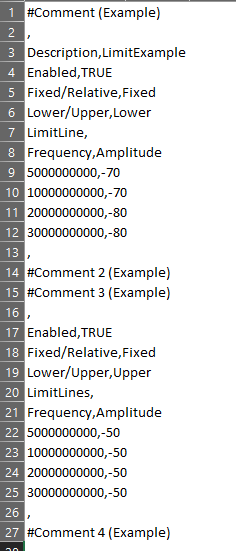
Description of Limit Line | Notes | |
|---|---|---|
#Comments start with “#” | Any row that begins with # is ignored by the FieldFox. | |
Description | LimitExample | Example “LimitExample” name only. Use any descriptive name. |
Bandwidth | 5000000 | Bandwidth values are required for Power Spectral Density (PSD) measurements which applicable to SA only. Learn more, see “Power Spectral Density (PSD) Function (SA mode Only)” on page 227. |
Unit | VPM/Hza | All parameters require “/Hz” added when using the SA mode’s PSD feature. Learn more, see https://rfmw.em.keysight.com/wireless/helpfiles/FFProgrammingHelpWebHelp/Home.htm. |
Enabled | TRUE | Choose: TRUE or FALSE |
Fixed/Relative | Fixed | Choose: Fixed or Relative |
Lower/Upper | Upper | Choose: Lower or Upper |
LimitLines | Must literally read: “LimitLines”. This indicates the limit line’s definitions begins below. | |
Frequencyb | Amplitudec | These must be written literally as “Frequency” and “Amplitude”. |
5000000000 | –70 | |
10000000000 | –70 | |
20000000000 | –80 | |
30000000000 | –80 | |
#Comment 2 (Example) | Any row that begins with # is ignored by the FieldFox. | |
#Comment 3 (Example) | Any row that begins with # is ignored by the FieldFox. | |
Enabled | TRUE | |
Fixed/Relative | Fixed | |
Lower/Upper | Upper | |
LimitLines | ||
Frequencyb | Amplitudec | |
5000000000 | –50 | |
10000000000 | –50 | |
20000000000 | –50 | |
30000000000 | –50 | |
#Comment 4 (Example) | Any row that begins with # is ignored by the FieldFox. | |
a.For PSD measurements, enter a Field Strength SCPI here. Learn more, see https://rfmw.em.keysight.com/wireless/helpfiles/FFProgrammingHelpWebHelp/SENSe_AMPLitude_UNIT.htm.
b.Fractional frequency values are OK (e.g., 50000000.99, etcetera). All values rounded to a resolution of 1 Hz.
c.Fractional amplitude values are OK (e.g., –49.99, –35.5, etcetera).
Figure 30-11 Example: Recalled Limit Line Formatting LimitExample.csv 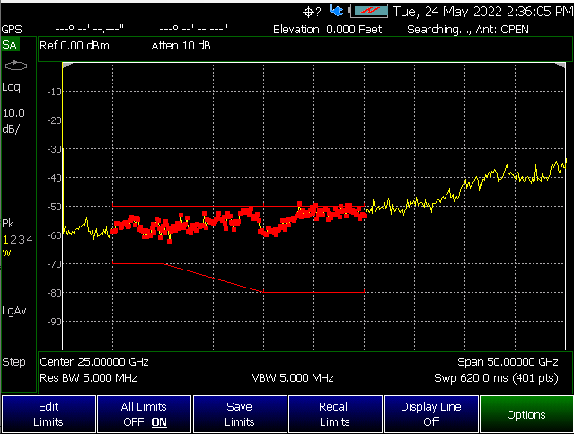
Display Line (I/Q, NF, and SA Modes Only)
A display line is a simple, horizontal line that can be placed at any amplitude level on the SA screen or set to any level in IQA. Use a display line as mental guide for visual feedback. A display line is similar to a Limit Line, except that no PASS/FAIL testing occurs. A display line is easier to create than a Limit Line. Learn more in “All about Limit Lines” on page 834.
Figure 30-12 Display Line with Annotations (SA mode shown, but others are similar)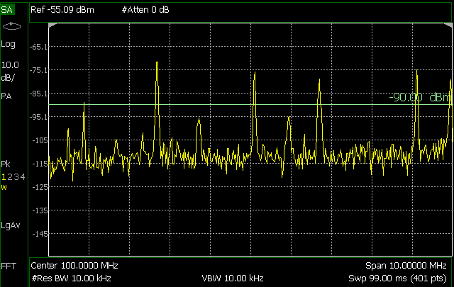
How to create and move a Display Line
1.Press Limit 8 > Display Line OFF ON
2.Then enter a Y-axis value using the arrows or the rotary knob, then press Enter. Or enter a value using the numeric keypad and press a suffix key or press Enter.
All about Trace Math
Trace Math is available in CAT (excluding DTF measurements), NA Mode, and FOPS (under USB Power Meter mode). Noise Figure (NF—Option 356) does not have trace math, but does have the ability to display data and memory traces. Refer to “How to display data and memory traces”.
A trace is a series of measurement data points that are connected to form a line. This ‘live’ data trace is updated as data points are measured.
A memory trace is a live trace that has been stored in the FieldFox volatile memory. It then becomes static, meaning it is not updated with measurements. It can be displayed on the screen by itself, or with a data trace for comparison purposes.
—In NA mode, memory traces are the same color as data).
—In CAT mode and FOPS, the data trace is displayed in yellow and the memory trace is displayed in blue.
How to display data and memory traces
1.Press Trace 6.
2.Press Math and Memory then Data->Mem to store the current live trace into memory. A ‘beep’ sounds to confirm the data trace has been saved to memory. There is no display annotation that indicates that the memory trace has been stored.
3.Then choose from:
—Press Data to view only the data trace.
—Press Memory to view only the memory trace.
—Press Data & Memory to view both the live trace and the stored memory trace.
Trace math is performed between a live trace and a memory trace. When one of the following math operations are selected, the yellow data trace displays the current measurement with the selected trace math applied. The math operation symbol indicated below in [brackets] is displayed on the lower left corner of the screen.
1.Press Trace 6.
2.If not already stored, press Data->Mem to store the current live trace into memory.
3.Then Data Math.
4.Then choose one of the following:
—Data + Mem [D+M] Current measurement data is added to the data in memory.
—Data – Mem D-M] Current measurement data is subtracted from the data in memory.
—Data / Mem [D/M] Current measurement data is divided by the data in memory.
—Math Off [Data] Displays trace data with NO math applied.
Data / Memory and Data - Memory math operations are performed on complex linear data before it is formatted. Because data is often viewed in log format, it is not always clear which of the two math operations should be used. Remember: dividing linear data is the same as subtracting logarithmic data. The following illustrates, in general, when to use each operation.
Use Data / Memory for normalization purposes, such as when comparing traces “before” and “after” a change is made or when measuring trace noise. In the following table, the Data/Mem values intuitively show the differences between traces. It is not obvious what Data-Mem is displaying.
Values to compare | Data/Mem | Data-Mem |
|---|---|---|
0.5 dB and 0.6 dB | 0.1 dB | –39 dB |
0.5 dB and 0.7 dB | 0.2 dB | –33 dB |
Use Data - Memory to show the relative differences between two signals. Use for comparison of very small signals, such as the S11 match of two connectors.
In the following table, Data/Mem shows both pairs of connectors to have the same 2 dB difference. However, the second pair of connectors have much better S11 performance (–50 and –52). The relative significance is shown in Data-Mem.
Values to compare | Data/Mem | Data-Mem |
|---|---|---|
–10 dB and –12 dB | 2 dB | –24 dB |
–50 dB and –52 dB | 2 dB | –64 dB |
All about Scale Settings IMPORTANT! Some of the scale settings do not apply to all of the modes.
Adjust the Y-axis scale to see the relevant portions of the data trace. The Y-axis is divided into 10 graticules.
This setting can be changed at any time without affecting calibration accuracy.
1.Press Scale / Amptd.
2.Then choose from the following three methods:
—Autoscale Automatically adjusts the Y-axis to comfortably fit the Minimum and Maximum amplitude of the trace on the screen.
—Set Scale, acquisition, and Reference Position:
—Scale Manually enter a scale per division to view specific areas of the trace.
—Ref Level Manually set the value of the reference line. Enter a negative value by pressing Run/Hold (+/-) either before or after typing a value.
—Ref Pos Manually set the position of the reference line. Values must be between 0 (TOP line) and 10 (BOTTOM line).
—Range Manually set the absolute power (dBm).
—Set Top and Bottom graticule values. The scale per division is calculated.
—Top to set the value of the Top graticule.
—Bottom to set the value of the Bottom graticule.
—Enter a negative value by pressing Run/Hold (+/-) either before or after typing a value.
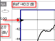
Scale annotation on the FieldFox screen Reference Line = red arrow Ref Level = –40 dB Ref Position = 1 Scale = 2 dB per division |
|
Averaging (CAT, NA, Power Meter, Channel Scanner, and Pulse Measurement Modes Only)
Trace Averaging helps to smooth a trace to reduce the effects of random noise on a measurement. The FieldFox computes each data point based on the average of the same data point over several consecutive sweeps.
Average Count determines the number of sweeps to average; the higher the average count, the greater the amount of noise reduction.
An average counter is shown in the left edge of the screen as Avg N. This shows the number of previous sweeps that have been averaged together to form the current trace. When the counter reaches the specified count, then a ‘running average’ of the last N sweeps is displayed. Average Count = 1 means there is NO averaging.
This setting can be changed at any time without affecting calibration accuracy.
Averaging is often used to increase the dynamic range of a measurement. To achieve the highest dynamic range, select NA mode and reduce the IF Bandwidth setting. Learn more about dynamic range in “Increase Dynamic Range” on page 118. |
How to Enable/Disable Averaging
1.Press BW 2 or Meas Setup 4 (Channel Scanner mode).
2.Then choose from:
—Channel Scanner: Average OFF ON change to ON to enable averaging (Default == OFF).
—Power Meter, Pulse Measurements: Average Auto Man OFF change to Auto or Man to enable averaging (Default == Auto, Auto == FieldFox sets the average count based on current mode settings).
—CAT, NA: Average 1 change to a number >1 to enable/set averaging (Default == 1 (OFF)).
3.Press Enter.
4.Refer to “How to set Trace Averaging” on page 853.
1.Press BW 2 or Meas Setup 4 (Channel Scanner mode).
2.Then choose from:
—Channel Scanner: Average Enable OFF ON change to ON to enable averaging and then set the current count or Time, using Average Count (Default == 10) or Average Timed (Default == OFF) softkey.
—Pressing the Average Count will allow to set a count for averaging. Average Count settings: Minimum count == 1 and Maximum count == 10000.
—Pressing the Average Timed will allow to set a time for averaging. Average Timed settings: Minimum time == 10 ms and Maximum time == 1000000s
When the Average Timed softkey is disabled (Default), averaging behaves normally using the Average Count softkey value. But, when Average Timed softkey is enabled, averaging continues until the specified time has elapsed and then the measurement will automatically hold. Pressing Run/Hold +/- to restart the measurement from 0s. For the Average Timed mode, press Run/Hold +/- before the averaging time has elapsed to pause time averaging and hold the measurement. Press Run/Hold +/- again to resume to continue time averaging and measurement.
—Power Meter, Pulse Measurements: Average Auto Man OFF change to Auto or Man to enable averaging (Default == Auto, Auto == FieldFox sets the average count based on current mode settings).
— Or set the current count, using the Num Averages softkey
—CAT, NA: Average 1 change to a number >1 to enable/set averaging (Default == 1 (OFF)).
3.Enter a value using the numeric keypad. Enter 1 for NO averaging.
4.Press Enter.
5.While Trace Averaging is in process, press Sweep 3 then Restart to restart the averaging at 1.