Learn more about NA Mode measurements in the FieldFox Supplemental Online Help: https://rfmw.em.keysight.com/wireless/helpfiles/FieldFoxOnlineSupplementalHelp/Home.htm.
See Also
Learn how to make 75Ω (ohm) Measurements in the Supplemental Online Help: https://rfmw.em.keysight.com/wireless/helpfiles/FieldFoxOnlineSupplementalHelp/Home.htm. |
Select NA Mode before making any setting in this chapter.
How to select NA Mode
1.Press Mode_.
2.Then NA.
S-parameters (scattering parameters) are used to describe the way a device modifies a signal. The FieldFox can measure four S-parameters. The syntax for each parameter is described by the following:
S22 | S11 (out | in)
out = FieldFox receiver port
in = FieldFox source port
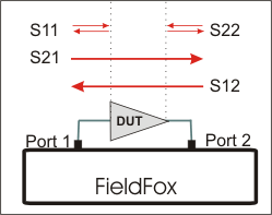
The FieldFox automatically switches the internal source and receivers to make both forward and reverse measurements. Therefore, the FieldFox can measure all four S-parameters with a single connection.
When the source comes from port 1, the measurement is said to be in the forward direction.
When the source comes from port 2, the measurement is said to be in the reverse direction.
S11 and S22 reflection measurements are used to measure the amount of reflections off the corresponding DUT port. Low reflections means there is a good impedance match between the source and DUT.
S21 and S12 transmission measurements are used to measure the loss or gain through a DUT over a specified frequency range. Both ends of the DUT must be connected to the FieldFox. The FieldFox signal source is transmitted out one of the test port connectors, through the DUT, and into the other test port connector
How to measure S-parameters
1.Press Preset then Mode Preset (Factory)
2.Press Measure 1 then choose from the following:
—S11 Reflection measurement at port 1.
—S21 Forward 2-port transmission measurement.
—S12 Reverse 2-port transmission measurement. May require an option.
—S22 Reflection measurement at port 2. May require an option.
OR select a multi-trace configuration. Learn more on “Multi-Trace Configurations” on page 101.
3.Press Freq/Dist then either Start and Stop or Center and Span to enter a Frequency Range for the measurement.
4.Press BW 2 then IFBW to select the IF Bandwidth for the measurement. Narrower bandwidths require more time to sweep, but lowers trace noise.
5.Press Sweep 3 then Resolution to select the number of data points for the measurement. More data points require more time to sweep.
6.Press Cal 5 to calibrate the measurement. Learn more in “How to Perform a Calibration” on page 134.
7.All other settings can be made AFTER calibration without compromising measurement accuracy.
In NA Mode ONLY, mixed-mode S-parameters (also known as Balanced measurements) are available with Option 212.
Because the FieldFox has only two test ports, only reflection measurements are available. Connect the balanced input or output of your DUT to the FieldFox ports 1 and 2
For highest accuracy, a Full 2-port calibration is required.
All FieldFox settings and features are supported (except Parameter Conversion) with mixed-mode S-parameters.
| Learn more about Balanced Measurements with the FieldFox in the FieldFox Supplemental Online Help: https://rfmw.em.keysight.com/wireless/helpfiles/FieldFoxOnlineSupplementalHelp/Home.htm. |
How to make mixed-mode S-parameter measurements
1.Press Measure 1.
2.Then More.
3.Then choose from the following:
—Scc11 Common reflect/common incident for logical port 1.
—Sdd11 Differential reflect/differential incident for logical port 1.
—Sdc11 Differential reflect/common incident for logical port 1.
—Scd11 Common reflect/differential incident for logical port 1.
To make balanced reflection measurements at the DUT output, connect the DUT output to the FieldFox ports.
In NA Mode ONLY, converts the active S-parameter trace to an equivalent impedance (Z), admittance (Y), or reciprocal 1/S-parameter
How to select parameter conversions
—Press Measure 1
—Then select an S-parameter
—Then More
—Then Conversion
—Then choose from the following:
—Off (default) No conversion is performed.
—Z Conv or Y Conv Perform conversion for impedance (Z) or admittance (Y). Then choose from the following for either:
——Auto The displayed S-parameter is converted to the appropriate Z or Y parameter: Refl for S11 and S22; Trans for S21 and S12. When the S-parameter is changed, the appropriate conversion changes automatically.
——Refl The displayed S-parameter is converted to Z or Y reflection, regardless of whether the S-parameter is reflection (S11 or S22) or transmission (S21 or S12).
——Trans The displayed S-parameter is converted to Z or Y transmission, regardless of whether the S-parameter is reflection (S11 or S22) or transmission (S21 or S12).
—1/S The displayed S-parameter is converted to 1/S-parameter.
In NA Mode ONLY, you can make unratioed, uncorrected receiver measurements. These measurements are typically used as diagnostic tools for service personnel. Receiver measurements are NOT corrected for absolute power. They are only useful for making relative measurements. The Y-Axis and markers are labeled in dB - NOT dBm. Specifically, R1 and R2, do NOT indicate the actual power levels out of the source ports.
How to make receiver measurements
—Press Measure 1
—Then More, then Advanced
—Then choose from the following:
A Port-1 test port (*1) | B Port-2 test port (*2) |
R1 Port-1 reference receiver (*1) | R2 Port-2 reference receiver (*2) |
(*) indicates the Auto-selected source port for the measurement | |
Source Port The FieldFox port to provide the source signal. Choose from the following: | |
—Auto The FieldFox sets the source port based on the selected receiver.
—Port 1 Select when measuring transmission at B receiver.
—Port 2 Select when measuring reverse transmission at A receiver.
Learn more about Raw Receiver Measurements at the FieldFox Supplemental Online Help: https://rfmw.em.keysight.com/wireless/helpfiles/FieldFoxOnlineSupplementalHelp/Home.htm.
In NA Mode you can display multiple traces on the FieldFox screen. 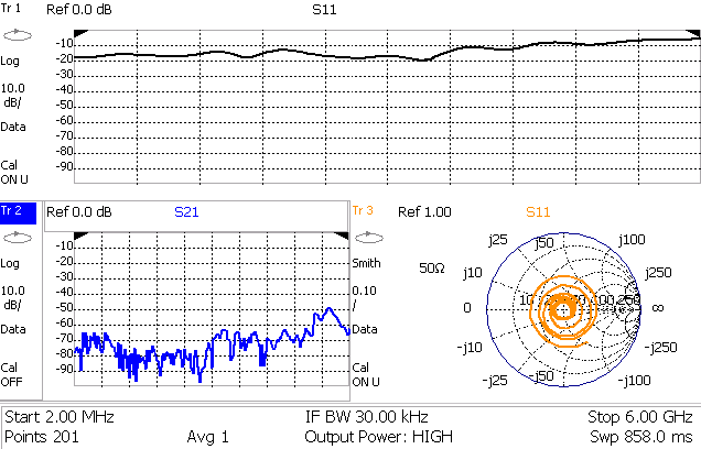
The graphic above shows a x3H configuration. Tr2 is the ACTIVE trace as indicated by the highlighted Tr2.
Trace Setting Notes
—The Frequency Range, IF BW, Resolution, Average, and Output Power settings are common for all displayed traces.
—All other trace settings, such as measurement, format, and limit lines, are applied individually to the ACTIVE trace in the same manner as when a single trace is present.
| IMPORTANT! For CAT and NA modes, limit lines do not apply |
—By default, a marker is created on ALL traces. However, they can be created individually by disabling Coupled Markers. Learn more in “Coupled Markers (NA Mode)” on page 822.
How to select a multi-trace configuration
1.Press Trace 6 > Num of Traces
2.Then choose from the following:
The default measurements depend on the options that are installed
| x1 | 1 trace standard configuration |
| x2 | 2 traces overlayed on a single graticule |
| x2H | 2 traces on separate graticules |
| x3H | 3 traces on separate graticules |
| x3 | 3 traces overlayed on a single graticule |
| x4 | 4 traces overlayed on a single graticule |
| x4H | 4 traces on separate graticules |


How to activate a trace in order to change a setting
—Use the  arrows OR
—Press Trace 6 then select Trace 1, Trace 2, Trace 3, or Trace 4, Only traces that are shown can be activated.
How to maximize the viewing of the active trace
1.Press System 7 > Full Screen.
2.Press any key to return to the standard display.
Both CAT and NA Modes allow you to view and change most relevant settings from a single location. All of these settings are discussed in this chapter and, unless otherwise noted, ALL of these settings can also be made using the standard softkey menus.
How to view and change Quick Settings
—Press Meas Setup 4 > Settings.
—Press Next Page and Previous Page to view all settings. If these softkeys are NOT available, then all available settings fit on one page.
—To change a setting:
—Use the arrows to highlight a setting.
—Then press Edit. The current setting changes to yellow.
—Some settings require you to press a softkey to change the value. Otherwise, use the numeric keypad, arrows, or rotary knob to change the value.
—When finished changing a value, press Done Edit.
—Press Dock Window to relocate the Settings table to a position relative to the trace window. The Dock Window setting persists through a Preset. Choose from the following:
—Full (Default setting) Only the Settings table is shown on the screen. The trace window is temporarily not shown.
—Left The Settings table is shown to the left of the trace window.
—Bottom The Settings table is shown below the trace window.
When finished changing ALL settings, press Done to save your settings.
NA Mode has a page specifically for making settings that pertain to Port Extensions, including Velocity Factor and Media Type.
Learn more in “Port Extensions” on page 114.
Learn more about Media Type in “Waveguide Calibrations” on page 147.
See also, Chapter 8 “Calibration for NA, CAT, and VVM Modes” and to “Apply Nearest (NA Mode Only)” on page 151.
How to view and change Calibration Settings
—Press Meas Setup 4.
—Then Calibration Settings
—Make these settings in the same manner as Quick Settings in the previous section.
Select the display format in which to present measurement results. This setting can be changed at any time without affecting calibration accuracy. Learn more about Display Formats in the FieldFox Supplemental Online Help: https://rfmw.em.keysight.com/wireless/helpfiles/FieldFoxOnlineSupplementalHelp/Home.htm.
The marker on screen readout can be changed to formats other than the display format. Learn more in “Marker Format” on page 824.
1.Press Measure 1 > Format [current setting].
2.Then choose from the following:
—Log Magnitude Displays magnitude in dB
—Linear Displays positive values only. Y-axis: Unitless (U) for ratioed measurements; Watts (W) for unratioed measurements.
—VSWR Used mainly for S11 and S22. Displays unitless reflection data.
—Phase Displays phase in degrees. The trace ‘wraps’ every 360 degrees, from +180 to –180, for easy scaling.
—Smith Used mainly for S11 and S22, which are plotted on a Smith Chart. Displays series resistance and reactance.
—More then…
—Polar Used mainly for S11 and S22. Displays magnitude and phase
of the reflection coefficient.
—Group Delay Used mainly for S21 and S12. Displays signal transmission (propagation) time through a device in seconds. The Group Delay aperture is the current Smoothing aperture. Default is 1.5% of the X-axis.
—Learn how to set Smoothing aperture on “Smoothing” on page 109.
—Learn more about Group Delay measurements at the FieldFox Supplemental Online Help: https://rfmw.em.keysight.com/wireless/helpfiles/FieldFoxOnlineSupplementalHelp/Home.htm.
—Real Displays only the real (resistive) portion of the measured complex data. The Y-axis is Unitless. Often used for Time Domain measurements.
—Imaginary Displays only the reactive portion of the measured complex data. The Y-axis is Unitless.
—Z Magnitude Displays the effective impedance in ohms.
—Unwrap Phase Same as Phase, but without 180 degree wrapping. Phase is unwrapped by comparing the phase from one data point to the next. If the phase difference between two data points is greater than 180 degrees, or if the phase of the first data point is greater than 180 degrees from DC, than the phase measurement is probably NOT accurate. To ensure that the phase measurement is accurate, increase the resolution setting. When making a narrow band measurement, reduce the start frequency for the unwrapped phase measurement to ensure the first data point is less than 180 degrees from DC.
Set the range of frequencies over which you would like to make measurements.
When the frequency range is changed after a calibration is performed, the calibration becomes interpolated. Learn more in “Interpolation *” on page 149.
—Press Freq/Dist
—Then choose from the following:
—Start and Stop frequencies – Specify the beginning and end of the sweep.
—Center and Span frequencies - Specify the center frequency and span of frequencies (half on either side of center).
—Follow each by entering a value using the numeric keypad, the arrows, or the rotary knob.
—After using the arrows or the rotary knob, press Enter. The increment setting of the arrows is based on the current span and can NOT be changed in NA Mode.
—After using the keypad, select a multiplier key. Learn more in “Multiplier Abbreviations” on page 53.
Adjust the Y-axis scale to see the relevant portions of the data trace. The Y-axis is divided into 10 graticules.
This setting can be changed at any time without affecting calibration accuracy.
1.Press Scale / Amptd.
2.Then choose from the following methods:
—Autoscale Automatically adjusts the Y-axis to comfortably fit the Minimum and Maximum amplitude of the trace on the screen.
—Autoscale All Autoscales all of the traces on the screen, useful only for multi-trace configurations.
—Set Scale, acquisition, and Reference Position
—Scale Manually enter a scale per division to view specific areas of the trace.
—Ref Level Manually set the value of the reference line. Enter a negative value by pressing Run/Hold (+/-) either before or after typing a value.
—Ref Pos Manually set the position of the reference line. Values must be between 0 (TOP line) and 10 (BOTTOM line)
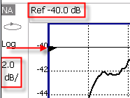
Scale annotation on the FieldFox screen —Reference Line = red arrow —Ref Level = –40 dB —Ref Position = 1 —Scale = 2 dB per division |
|
Magnitude Offset allows you to offset the magnitude (not phase) data by a fixed and/ or sloped value in dB. If the display format is Linear Magnitude or Real (unitless), the conversion from dB is performed and the correct amount of offset is implemented.
The Magnitude offset setting affects only the active trace.
How to set Magnitude Offset
1.Press Scale / Amptd
2.Then More
—Then Magnitude Offset - Offsets the entire data trace by the specified value.
—Then enter a positive or negative offset value in dB using the numeric keypad, the arrows, or the rotary knob. Press a multiplier key. Learn about multiplier abbreviations.
—And/or press Slope - Offsets the data trace by a value that changes linearly with frequency. The offset slope begins at 0 Hz. and continues to the stop frequency. The offset value at the start frequency is then calculated from 0 Hz.
—Then enter a positive or negative offset slope value in dB/GHz using the numeric keypad, the arrows, or the rotary knob. Press a multiplier key. Learn about multiplier abbreviations in “Multiplier Abbreviations” on page 53.
Electrical delay is a mathematical function that simulates a variable length of lossless transmission line. Use the electrical delay feature to compensate for the linear phase shift through a device and view only the deviation from linear phase of the device.
You can set the electrical delay independently for each measurement trace. To apply an electrical delay to all measurement traces, use Port Extensions. Learn how in “Port Extensions” on page 114.
Learn how to set Phase formats in “Phase Offset” on page 107.
How to set Electrical Delay
1.Press Scale / Amptd > More > Electrical Delay
2.Enter a time value using the numeric keypad, the arrows, or the rotary knob.
3.Press a multiplier key. Learn about multiplier abbreviations in “Multiplier Abbreviations” on page 53.
Electrical Delay can also be set using the Mkr->Delay feature. Learn how on “Marker Functions” on page 832.
Phase offset mathematically adjusts the phase measurement by a specified amount, up to 360°. Use this feature in the following ways:
Improve the display of a phase measurement. This is similar to the way you would change the acquisition in an amplitude measurement. Change the phase response to center or the response on the screen.
Emulate a projected phase shift in your measurement. For example, if you know that you need to add a cable and that the length of that cable will add a certain phase shift to your measurement, you can use phase offset to add that amount and simulate the complete device measurement.
You can set the phase offset independently for each measurement trace.
How to set Phase Offset
1.Press Scale / Amptd > More > Phase Offset
2.Enter a value in degrees using the numeric keypad, the arrows, or the rotary knob. Press Enter.
Averaging helps to reduce the effects of random noise on a measurement. You specify the number of measurements to be averaged. The more measurements averaged, the greater the amount of noise reduction. An average counter is shown in the left edge of the screen as Avg <n> where <n> is the number of measurements that are averaged.
Averaging can be set before or after calibration. When set before calibration, each calibration standard is measured <n> times and averaged. More time is needed to perform the calibration, but there will be less noise in the resulting error terms which means that subsequent measurements will also have less noise. In addition, noise is further reduced by continuing to average after calibration.
1.Press BW 2.
2.Then Average <n> where <n> is the number of measurements to average.
3.Enter a value using the numeric keypad. Enter 1 for NO averaging.
4.Press Enter.
5.Then Average Mode Choose from the following:
—Sweep - Each data point is based on the average of the same data point being measured over <n> consecutive sweeps. The average counter shows the number of previous sweeps that have been averaged together to form the current trace. When the counter reaches the specified count, then a ‘running average’ of the last <n> sweeps is displayed.
—Point - Each data point is measured <n> times and averaged before going to the next data point. On subsequent sweeps, averaging restarts by measuring each data point again <n> times. The average counter is not updated because data is not displayed until all the averages have been applied.
—Point averaging is usually faster than sweep averaging. However, you may need to increase the Point Average count to obtain the same level of noise reduction as with sweep averaging.
6.While averaging is in process, press Sweep 3 then Restart to restart the averaging at 1.
The FieldFox converts the received signal from its source to a lower intermediate frequency (IF). The bandwidth of the IF bandpass filter is adjustable. Reducing the IF receiver bandwidth reduces the effect of random noise on a measurement. However, narrower IF bandwidths cause longer sweep times.
How to set IF BW
1.Press BW 2 > IF BW
2.Then choose from the following:
—10 Hz | 100 Hz | 1 kHz | 10 kHz | 100 kHz
More 30 Hz | 300 Hz | 3 kHz | 30 kHz
Trace smoothing averages a number of adjacent data points to smooth the peak-to-peak noise values on a displayed trace. The number of adjacent data points that are averaged is known as the smoothing aperture. Aperture is set by specifying a percentage of the X-axis span.
Trace smoothing does NOT significantly increase measurement time.
Smoothing is used in Group Delay measurements, although it can be used with any NA format EXCEPT Polar or Smith Chart. Learn more about NA Mode formats, including Group Delay, in “Format” on page 104.
When enabled, Smo appears on the FieldFox screen.
How to set Smoothing
1.Press BW 2 > Smoothing ON OFF
2.Then Sm. Aperture and enter a value between 0 and 25 (percent) using the numeric keypad.
3.Press Enter
This setting determines whether the FieldFox sweeps continuously or only once each time the Single button is pressed. Use Single to conserve battery power or to allow you to save or analyze a specific measurement trace.
This setting can be changed at any time without affecting calibration accuracy.
How to set Single or Continuous
1.Press Sweep 3.
2.Then choose one of the following:
—Single Automatically sets Continuous OFF and causes FieldFox to make ONE sweep, then hold for the next Single key press. Hold is annotated in the upper left corner of the display when NOT sweeping, and changes to an arrow --> while the sweep occurs.
—Continuous Makes continuous sweeps. This is the typical setting when battery power is not critical.
—You can also use Run / Hold +/- to toggle between Single and Continuous.
Resolution (Number of Data Points)
Data points are individual measurements that are made and plotted across the X-axis to form a trace. Select more data points to increase measurement resolution. However, more data points also takes more time to complete an entire measurement sweep.
When the Resolution is changed after a calibration is performed, the cal becomes interpolated. Learn more in “Interpolation *” on page 149.
1.Press Sweep 3 > Resolution.
2.Then choose from the following:
101 |201 | 401 | 601 | 801 | 1001 | 1601 | 4001 | 10001.
Using SCPI, or measurement quick settings table, Resolution can be set to ANY number of points between 3 and 10001. See the Programming Guide Help: https://rfmw.em.keysight.com/wireless/helpfiles/FFProgrammingHelpWebHelp/Home.htm. Learn more, “Quick Settings Table” on page 102.
The fastest possible sweep time is always used as the default setting. Use the Min Swp Time setting to slow the sweep time when measuring long lengths of cable. Learn more at the FieldFox Supplemental Online Help: https://rfmw.em.keysight.com/wireless/helpfiles/FieldFoxOnlineSupplementalHelp/Home.htm.
The actual sweep time is shown on the FieldFox screen. See the Screen Tour on “Screen Tour” on page 51. To increase the sweep time, enter a value that is higher than the actual sweep time. The increase will not be exactly the amount that you enter, as the actual sweep time is the composite of many factors.
| Measurement speed specifications do NOT apply in Temperature Control Mode. Learn more in “Temperature Control Mode” on page 36. |
1.Press Sweep 3.
2.Then Min Swp Time.
3.Enter a value using the numeric keypad.
4.Press a multiplier key. Learn about multiplier abbreviations in “Multiplier Abbreviations” on page 53.
External triggering (NA and SA modes ONLY) allows you to initiate a sweep when an external DC voltage is sensed at the Ref In/Trig In connector on the FieldFox top panel. See External Triggering for SA Mode in “Triggering” on page 206.
Trigger Source
1.Press Sweep 3 > Trigger > Trig Source
2.Then choose from the following:
—Int (Internal) Sweeps are initiated by the FieldFox internal circuitry. When Sweep is set to Continuous, a new sweep begins automatically when the previous sweep ends.
—Ext (External) A sweep is initiated on the rising or falling edge of an external TTL signal at the Ref In/Trig In connector on the FieldFox top panel.
—When the FieldFox is armed for an external trigger signal, Wait is annotated on the display.
—A sweep can NOT be initiated by an external signal while a sweep is in progress.
—A sweep can NOT be initiated by an external signal when in HOLD mode. Learn more about HOLD mode in.
—Pnt (Point) An external trigger type that acquires exactly one point per trigger input. To ensure triggers are recognized and processed in order, use the external trigger output function to indicate when the FieldFox is ready for another input trigger. Alternatively, slow the external triggers coming in from external equipment to a rate where FieldFox does not miss a trigger. The External Trigger output signal is only selectable when Point Mode Trigger is enabled. Not supported in other trigger modes. External Trigger output signal is sent as soon as FieldFox has processed the last trigger signal that was detected. As each point is acquired, the data will show up on screen. If a trigger has not been detected, a yellow Wait indicator will show on the sweep status icon area.
—When the FieldFox is armed for an external trigger signal, Wait is annotated on the display.
——A sweep can NOT be initiated by an external signal when in HOLD mode. Learn more about HOLD mode in.
Error Handling and Recovery
—Point Mode trigger is not compatible with sweep setups that require forward and reverse sweeps such as:
—Full 2port cal
—Cal ready (Full 2Port)
—Multiple displayed parameters that include the requirement for forward and reverse sweeps such as S11 and S22 together on the display
— When point mode trigger is already enabled, if conditions are changed requiring forward and reverse sweeps, an error "Error: Point trigger not compatible with 2-port cal." will be displayed and point mode trigger will revert to Internal trigger. This includes turning on a CAL that requires forward and reverse sweeps or displaying multiple parameters that would require forward and reverse sweeps.
— If the FieldFox is in a state requiring two sweeps and the user selects point mode triggering, an error "Error: Point trigger not compatible with 2-port cal." will be displayed and point mode trigger will revert to Internal trigger.
Trigger Slope
Determines which edge of an External trigger signal initiates a sweep.
1.Press Sweep 3 > Trigger > Trig Slope
2.Then choose from the following:
—Positive Sweep is initiated by the rising edge of signal at about 1.7V.
—Negative Sweep is initiated by the falling edge of signal at about 1.0V.
Set the power level out of the FieldFox to High, Low, or manually set power level to a value between High and Low.
Generally, the high power setting is used when measuring passive, high-loss devices to place the signal farther from the noise floor. However, for devices that are sensitive to high power levels such as amplifiers, use the Low power setting.
For best measurement accuracy, use the Manual power setting at -20 dBm. After calibration, the power level can be decreased for amplifiers, or increased for higher dynamic range.
| Power Level settings in this mode will NOT change Power Level settings in other modes. To help prevent damage to your DUT, use caution when changing modes with your DUT connected to the FieldFox test ports. |

| For consistency with other FieldFox A/B models (backward compatibility), the default Output Power is set to –15 dBm. To avoid overload when using FieldFox C model, users should manually change the Output Power setting to –20 dBm. |
1.Press Meas Setup 4.
2.Then Output Power
—High Sets output power to the maximum achievable power at all displayed frequencies. Output power is NOT FLAT across the displayed FieldFox frequency span. Please see “Specifications/Data Sheet” on page 979 for expected power levels.
—Low Sets output power to approximately –50 dBm, FLAT across the displayed FieldFox frequency span.
—Man (default setting at -15 dBm) Set output power to an arbitrary value, FLAT across the displayed FieldFox frequency span. If flattened power can NOT be achieved, a warning message and beep occurs. To achieve a flattened output power, reduce the power level or stop frequency.
a.Then press Power Level
b.Then enter a value using the numeric keypad, the arrows, or the rotary knob.
c.Press Enter.
To accurately view data presented in Smith Chart format, first set the System Impedance.
Learn how to select Smith Chart format in “Format” on page 104.
Learn how to make 75Ω measurements at the FieldFox Supplemental Online Help: https://rfmw.em.keysight.com/wireless/helpfiles/FieldFoxOnlineSupplementalHelp/Home.htm.
How to set System Impedance
1.Press Meas Setup 4 > Settings.
2.Then scroll to System Z0 and press Edit
3.Then type either 50 or 75 and press Enter
Port extensions allow you to electrically move the calibration reference plane on either port 1 or port 2 after you have performed a calibration.
Why use Port Extensions
Use port extensions if you are unable to perform a calibration directly at your device because the location is not accessible. Perform a calibration at a convenient place, then use port extensions to compensate for the time delay (phase shift) to the desired reference plane. On the FieldFox, port extensions does not compensate for the loss of the additional electrical length, nor any mismatch errors beyond the calibration reference plane.
Also, use port extensions if you have already performed a calibration, and then decide that you need to add a length of transmission line in the measurement configuration. Use port extensions to “tell” the FieldFox that you have added the length to a specific port.
—With S11 and S22 reflection measurements, the FieldFox doubles the port extension valued that you enter to account for the additional delay in the forward and reverse directions.
—With S21 and S12 transmission measurements, the port 1 and port 2 extensions are added together. This accounts for the total transmission delay going through ports 1 and 2.
Port extensions and Electrical Delay differ in the following ways:
—Electrical delay applies to a specific trace
—Port extensions apply to specific hardware ports
Port Extensions and Electrical Delay can be set independently. When both are set, the delay adds together. Learn more about Electrical Delay in “Electrical Delay” on page 107.
How to apply Port Extensions
1.Press Meas Setup 4 > Port Extensions > Port Extensions ON > Port1 Extension
2.Then enter time value using the numeric keypad, the arrows, or the rotary knob. Press Enter or select a seconds (time) multiplier.
You can also set Port Extensions by pressing Meas Setup 4 then Calibration (settings).
While setting Port Extension, the physical length of the extension, at the current Velocity Factor setting, is visible to the right (red box in above image).
The electrical delay or port extension value is entered as delay, or electrical length, in units of time.
Entering the velocity factor causes the FieldFox to accurately display the equivalent physical length in meters (NOT available in feet) that corresponds to the entered electrical delay.
Velocity factor is the ratio of the velocity of wave propagation in a coaxial cable to the velocity of wave propagation in free space. This velocity depends on the relative permittivity of the cable dielectric (er).
Velocity factor = 1/sqrt(er)
VF = 0.66 corresponds to wave propagation through a polyethylene dielectric.
VF = 1.0 (default setting) corresponds to wave propagation through free space (a vacuum).
How to set Velocity Factor
1.Press Meas Setup 4 > Port Extensions > Velocity Factor
2.Then enter a value between 0.1 and 1 using the numeric keypad, then press Enter.
You can also set Velocity Factor by pressing Meas Setup 4 then Calibration (Settings).
Big Marker Display States (A and B)
This feature, available ONLY in NA Mode, allows you to view up to three Big or Super Big marker readouts. This is done by using up to two different display states called A and B. Each display state is comprised of the settings listed below. When the Big Readout setting is toggled through A and B, these display states are recalled.
How to create Big Marker Display States
To have big readouts, markers MUST be created using the following procedure.
If you have already set up your display and do not want to lose it, then save the current state to a state file. Learn how in “State Files” on page 918. The following procedure will overwrite your display state.
—Press Mkr ->/ Tools
—Then Big Readout
—A or B - The A or B display state is recalled. If none have been defined, then the default display state is recalled.
—OFF - The B display state is visible but without the Big Marker Readout.
—With A or B selected, then press Edit Big Marker (A or B)
—Then edit the following display state settings:
—Num Traces – Choose the Multi-Trace configuration x1, x2, or x3. Only Overlayed configurations are allowed. Learn more in “Multi-Trace Configurations” on page 101.
—Font Size – Choose either Big or Super Big. Super Big marker readout #3 will cover some of the measurement grid.
—Trace Settings - For each possible trace (1, 2, and 3) select from the following:
—Measurement – S-parameter or Receiver measurement to display. S11 is default. Learn more in “About S-parameters” on page 97.
—Meas Format – Log is default. Learn more in “Format” on page 104.
—Bandwidth (ON) – Marker readout for marker bandwidth search. OFF is default. Learn how to set BW parameters in “How to Search with Markers” on page 825.
—Big Readout - For each marker readout (1, 2, and 3), select from the following:
—Marker # - Enter a number from 1 to 6 to create the marker. 1 is created by default.
—Trace # - The marker# is created on this trace. Tr1 is selected by default. The corresponding Num Traces must first be selected. For example, to create a marker on Trace 3, first select Num Traces = x3.
—Format – Format for the marker readout. Select Default to make the marker readout format the same as the display format. Default is selected by default.
—Mkr Tracking – ON: Select the parameter to track on the standard Marker Search menu. OFF is selected by default. When set to ON, Peak tracking is set by default. Learn about Marker Tracking in “Marker Functions” on page 832.
—State – Choose from Normal, Delta, or OFF. The default marker (1) is created in Normal. Learn more in “Marker Functions” on page 832.
—Enabled – Turns the Big Readout of the corresponding marker ON and OFF. The default marker (1) is set ON by default. —To move a marker, press Marker, then Marker, then scroll to the marker number to be moved. The new marker position can NOT be saved with the A or B display state. — Settings that are NOT listed above are NOT affected by the recalled display states. — Changes to the above settings outside the Big Readout menu will be overwritten when Big Readout (A or B) is selected. For example, suppose the display format for the B state is Log. If you change the display format to Lin using the standard menu (Meas 1, Format), the setting will show on the display. But if you then use the Big Readout (A | B | OFF) setting, when B is recalled, the Lin setting will be overwritten with the original Log setting.
Dynamic range is the difference between maximum input power to the FieldFox receiver (without compressing the receiver), and the minimum measurable power (noise floor). Measurement accuracy is increased when the DUT response is at least 10 dB above the noise floor. For a measurement to be valid, input signals must be within these boundaries. 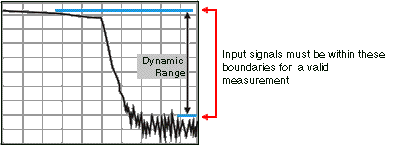
The following settings will increase the dynamic range of your NA mode measurement.
—Increase Power Level: Press Meas 4 then Output Power High
—Lower the IFBW: Press BW 2 then IF BW
—Increase Averaging: Press BW 2 then Average
The following procedure MAY increase the dynamic range of your NA mode measurement. The results you see will depend on the performance of your DUT.
With an S21 trace active:
1.With RF OUT (port-2) open, press Trace 6 then Math and Memory then Data->Mem
2.Re-connect the DUT.
3.Press Data Math then Data-Mem