11IQ Analyzer (IQA) – Option 351
IQA mode measures signals at the SA RF IN connector.
IQA mode requires the FieldFox to have SA mode installed. IMPORTANT! 85571A-028 (28 GHz 5G Phased Array Antenna) accessories not suitable for use in wet locations. The FieldFox can be used with both VDI and OML frequency extender. Refer to “Utilities” on page 862, the Configuration Guide at: https://www.keysight.com/us/en/assets/3125-1447/configuration-guides/FieldFox-Handheld-Analyzers-D-models.pdf, and to “Contacting Keysight” on page 5.

Figure 11-1 IQ Analyzer (IQA) Display - LTE–TDD signal captured using the FieldFox’s I/Q analyzer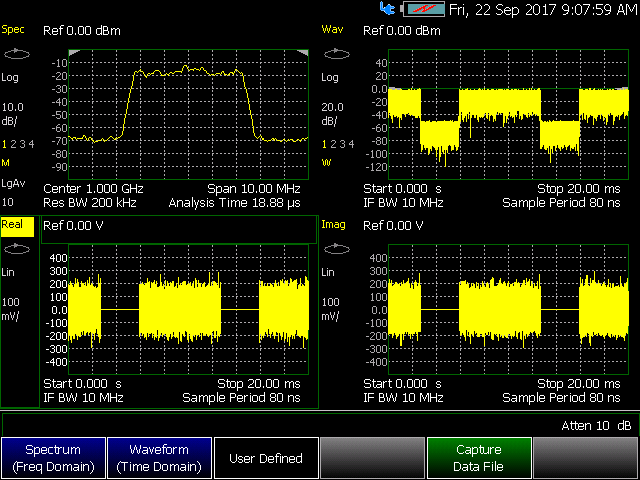
Figure 11-2 IQ Analyzer (IQA) Display - Window Shape Flat Top spur free 1 GHz center frequency (span=100 MHz) captured using the FieldFox’s I/Q analyzer (Requires Option B10)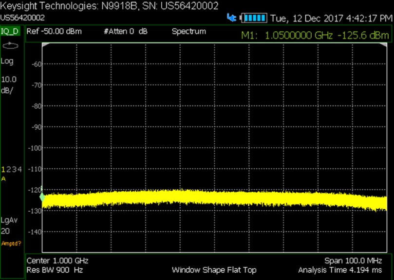
—“How to Make Measurements Using the I/Q Analyzer Mode” on page 315 |
—“How to Make Independent Source Settings and Pulse Generator Tracking” on page 317 |
—“How to modify the I/Q data measurement parameters” on page 323 |
“Other Features Available” on page 341 —Constellation and Frame Summary – “IQ Analysis Streaming (SA Mode Only)” on page 263 —External Gain (SA chapter) – “External Gain” on page 166 —Display lines (SA chapter) –“Display Line” on page 226 —Limit Lines (Data Analysis chapter) – “All about Limit Lines” on page 834 |
See Also
About I/Q Analyzer (IQA) Measurements
The I/Q Analyzer Mode makes general purpose frequency domain and time domain measurements. The mode enables two types of I/Q measurements:
—frequency domain and
—time domain measurements Noise level in time-domain measurements are higher for IF-BW >100 MHz due to raised noise levels at the edges of the 120 MHz bandwidth.
In order to ensure consistent results between frequency domain and time domain, spectrum measurement and waveform measurement are based on the same I/Q acquisition. The following acquisition parameters are automatically calculated to satisfy these requirements:
1. RBW and IF BW specified in Spectrum measurement BW (BW 2) menu.
2.Start time and Stop time specified in Waveform measurement Sweep (Sweep 3) menu and IF BW specified in Waveform measurement BW
(BW 2) menu. See also, “Setting the IF Path” on page 314
3.I/Q signal capture related parameters specified in the Measurement Setup (Meas Setup 4) menu. See also, “Setting the IF Path” on page 314
Some measurement parameters are auto-coupled and are not user-settable.
How to check or set the IF Path. By default the IF Path is set to Auto.
1.Press Meas Setup 4
2.Press BW 2.
3.Then IF Path The underlined setting is the current setting. Choose Auto, 10 MHz, or 100 MHz (100 MHz requires Option B04 or B10 and either Option 350 RTSA or Option 351 IQ Analyzer).
Optional: After you click 100 MHz, you can use the Freq/Dist hard key and the number pad or using the numeric keypad, the  arrows, to increase your IF path bandwidth to 120 MHz.
When in full span, ADC dither raises the noise floor at the edges of the 120 MHz. |
I/Q Analyzer (IQA) Mode Settings
| When you initially select I/Q Analyzer, Real-Time SA, or some of the other spectrum settings (such as center frequency) a factory channel Equalization measurement is applied to the signal. During channel equalization measurement, the FieldFox displays a “Start Channel Equalization”. Stopping channel equalization is not permitted. See also, “Alignments” on page 219, in Chapter 9, “SA (Spectrum Analyzer) Mode (Option 233–Mixed Analyzers).” |
Select IQA Mode before making any settings in this chapter.
How to select IQA Mode
—Press Mode_.
—Then More (may not be available—number of installed options dependent)
—Then IQ Analyzer.
How to Make Measurements Using the I/Q Analyzer Mode
The Measure menu is used to set common parameters, predefined views selection, and measurement switching.
Spectrum has only one predefined view and Waveform measurement has two predefined views. There is a User Defined measurement, which can be used to display up to four different views (windows) simultaneously on the display screen. You can select which type of data to display in each of the views from the Trace menu.
See also, “How to Capture I/Q Data to a File” on page 320 and “Setting the IF Path” on page 314.
1.Press Preset then Mode Preset (Factory)
2.Press Measure 1 then choose from the following:
—Spectrum (Freq Domain) (Default) – Selects frequency spectrum as the current displayed measurement.
—Waveform then choose one of the following:
—RF Envelope Selects log RF envelope in time domain (default). Noise level in time-domain measurements are higher for IF-BW >100 MHz due to raised noise levels at the edges of the 120 MHz bandwidth.
—IQ Waveform Selects linear Real and imaginary I/Q waveform values.
—User Defined Selects a default user defined 4-quadrant display showing the following data:
—Log magnitude of the spectrum of the I/Q data versus frequency
—Log magnitude of the I/Q data (RF Envelope) versus time
—The real component of the I/Q data versus time
—The imaginary component of the I/Q data versus time
The user defined measurement can be modified to change the number of displays from 4 to 3, 2, or 1.
—Source Opens a softkey menu for Independent Source and Source Tracking settings. This softkey menu is only available for B/C model equipped with Pulse Generator license (Option 357) and operating in IQA mode. Refer to “How to Make Independent Source Settings and Pulse Generator Tracking” on page 317
—Capture Data File Opens a menu to enable saving I/Q data to a file. When you press the Start capture softkey the data is saved to a file and the default file IQDataFile.csv is stored in the internal memory. Refer to “How to Capture I/Q Data to a File” on page 320.
How to Make Independent Source Settings and Pulse Generator Tracking
For best results, when using the independent source feature, all alignment and the battery saver features should be turned off. Refer to “All Alignment and Align All Now” on page 222 and “Preferences” on page 870 |
This feature may require an option. For a comprehensive list, view the FieldFox Configuration Guide at: https://www.keysight.com/us/en/assets/3125-1447/configuration-guides/FieldFox-Handheld-Analyzers-D-models.pdf.
Independent Source can be enabled in IQA mode for B/C model with Pulse Generator license (Option 357).
To view the internal source, you must connect a cable or device between the RF Output connector and the RF Input connector.
The Pulse Generator Tracking feature required Option 357, allows the Independent Source tracking to effectively retain the settings from the most recent activity, specifically when the Pulse Generator mode was last used with RF enabled.
To utilize Pulse Generator Tracking feature, users should navigate to the Pulse Generator, configure a signal and ensure that RF is set to ON. Learn more in Chapter 24, “Pulse Generator Mode – Option 357”, on page 653
—Press Measure 1 > Source
—Source Enable ON OFF
—ON Turns ON the internal source.
—OFF Turns OFF the internal source.
—Source Tracking Choose from the following:
—OFF The source is set to a CW frequency independent from the SA settings. Srcw is annotated on the screen.
—Center Freq The source is set to a CW frequency, but that frequency “tracks” the SA receiver Center Frequency settings. Therefore, the signal always appears at center of the display. Srcp is annotated on the screen.
—Pulse Gen Only available for B/C model equipped with Pulse Generator license (Option 357) and operating in IQA mode. Track the pulse generator signal to replicate the same signal setup established in Pulse Generator mode. SrcPg is annotated on the screen.
Pulse Gen softkey appears greyed out and cannot be selected despite having Option 357 on B/C model. Refer to Figure 11-3 on page 319. This occurs because the signal has not been configured with RF ON within the Pulse Generator mode. Learn more in Chapter 24, “Pulse Generator Mode – Option 357”, on page 653. |
—Source Power Sets the source power level. Choose from:
—Leveled Enter a value from –60 dBm to 10 dBm using the numeric keypad, arrows, or the rotary knob1. The source power is reasonably flat across the frequency span.
—MAX The power level is set to the maximum achievable power level at each frequency.
—Source CW Freq Sets the CW frequency that is used.
When Source Enable is ON, Source CW Freq softkey is enabled ONLY when Source Tracking is set to OFF. |
When Source Tracking is set to Pulse Gen, Source Power and Source CW Freq are disabled and cannot be adjusted. The Source CW Freq reveals the RF Freq relayed from the Pulse Generator mode. Refer to Figure 11-4 on page 319 and Figure 11-5 on page 319 for track the Pulse Gen example. |
The Independent Source output signal may be momentarily interrupted for automatic SA Receiver alignments or Battery Saver functionality. |
To prevent automatic alignments from interrupting the source, turn off all alignment. Refer to “How to Access Individual Alignments” on page 223.
—Press Cal 5
—Then press All Alignment and select OFF or Hold to disable All Alignment
To prevent Battery Saver from interrupting the source, turned off Battery Saver. Learn more in “Battery Saver” on page 873.
—Press System 7 > Preferences > Preferences
—Then in the table, select Battery Saver value column and press Edit
—Then press Battery Saver to toggle OFF to disable Battery Saver
Figure 11-3 Softkey Menu: Pulse Generator Not Configured (RF OFF) - Pulse Gen Greyed out
Figure 11-4 Softkey Menu: Pulse Generator Configured (RF ON) - Pulse Gen Enabled
Figure 11-5 Track the Pulse Gen in IQA mode Examples - Modulated Signal Setup Using Pulse Generator Mode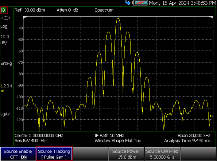
How to Capture I/Q Data to a File
There are two I/Q data file count capture modes, Single and Multiple. To capture your IQA data measurements:
—Press Measure 1 > Capture Data File then choose one of the following:
— File Settings Opens a menu to set the file choices:
——File Count File count can be set to Single or 1 (all data saved into a single file for the current displayed data) or Multiple. When using Multiple as the file count, the user can enter the number of files to save, and the FieldFox is auto-coupled to Continuous acquisition mode and to Multiple capture and all data is saved to either an external SD card or USB storage device. Each acquisition is saved, before the next data acquisition occurs. (default: 1, minimum: 1, maximum: 1,000,000,000)
——Single capture example (default): IQDataFile.csv
——Multiple capture (default):
Example is: IQDataFile_20171031 14.33.26.1050.csv).
(format is: IQDataFile_yyyymmdd hh.mm.ss.ffff.csv).
——Refer to the Start softkey on page 321 and to the “Example:” on page 321.
——File Type Selects the format of the output data file (CSV, TXT, SDF, or MAT). (Default: CSV)
——Device Selects the storage location for your data files (Internal, SD Card, or USB). Internal is not available, if the File Count is set to Multiple (default: Internal).
If you do not have an external device connected and attempt to save your data, a warning message is displayed: "Warning: Only an external storage device can be used in multiple file mode."
Then select:
——Internal (default) Selects the internal memory of the FieldFox as the storage location for all data files. Internal is only available when File Count is set to Single.
——SD Card Selects the external SD card slot as the storage location for all data files.
——USB Selects an external USB storage device as the storage location for all data files.
——Filename Opens a file manager Labeler menu that enables you to customize your data filenames. Refer to “File Management” on page 913 (default: IQDataFile).
——Back Returns to the previous softkey menu.
—Capture Settings then choose one of the following:
——Capture Time Sets the length of the I/Q trace capture time (default: 100 ms, range: 80 ns to dynamic (i.e., Maximum capture time is 1.07374s, which is associated with a sample rate of 125 MHz)).
——Sample Rate Sets the I/Q data sample rate value (default: 125 MHz, maximum: 125 MHz, couplings: 1.25 * IF Bandwidth).
——Sample Period Sets the 1/Sample Rate value (default: 8 ns, maximum: 80 ms, couplings: Sample Rate).
——Capture Samples Sets the capture length using a sample number (default: 12501, minimum: 1, maximum: 134217728, couplings: Capture Time).
——Back Returns to the previous softkey menu.
—Start Starts the I/Q data capture and stores the data into a default file and location (internal). Filenames and storage location can be customized. See also, the “Example:” on page 321 and to Chapter 33, “File Management.”
——Refer to the File Count softkey on page 320.
—Stop immediately stops the I/Q data file capture and stops writing data to the current I/Q data file (no data is saved). If the I/Q data was being saved when the Stop softkey is pressed, the file is deleted. Refer to “Example:” on page 321.
Single:
——If the Capture Time is set to 100 µs, and you press the Start softkey, in Single mode the FieldFox saves 100 µs of the current I/Q data.
Multiple:-
——If the File Count is set to 200, and you press the Start softkey, the FieldFox saves your 200 I/Q data files and stops. The I/Q data files are saved into 200 files similar to:
IQDataFile_yyyymmdd hh.mm.ss.ffff.csv.
——If you press Stop, before the 200 I/Q data files have been saved, the FieldFox stops (interrupts) the multiple I/Q data file saving at the number of the current file. So, if you press Stop on file number 175, the saving process stops. If file number 175 has not been saved, it is deleted. But, I/Q data files 1 through 174 that have been saved prior to pressing Stop, are still saved for reference.
See also, Chapter 33, “File Management.”
How to modify the I/Q data measurement parameters
The following sections assume you have already selected your I/Q data measurement type (i.e., Spectrum, Waveform (RF Envelope or I/Q Waveform), or User Defined).
“Changing between the Continuous and Single captures and adjusting the Trigger settings” on page 325 |
Adjusting the Bandwidth Settings
—Press BW 2.
—Then choose from the following:
—Res BW (Spectrum only) – Sets the resolution bandwidth of the FFT analysis. Changing this value changes the FFT window size, analysis length, and the sweep time (data acquisition capture length). This softkey is only available when IQA is set to Spectrum (Freq Domain). When the resolution bandwidth value is set to Auto (default) the FieldFox automatically sets the optimum resolution bandwidth value.
(Default: 100 Hz, Minimum: 10 Hz, maximum: 100 MHz).
| There is a significant difference between resolution BW in FFT measurements and the resolution BW of a traditional “sweeping” spectrum analyzer (SA) measurement. The resolution BW in FFT measurements does not directly control the IF BW like a traditional SA swept measurement. Resolution bandwidth is directly related to the analysis length (window) and or data acquisition capture length (sweep time). |
—Analysis Length Sets the FFT analysis length that is the length of the complex I/Q data points (I/Q–pairs) vector that is used for spectrum analysis, expressed in the number of samples. (Couplings: In Auto, this setting is directly coupled to the Res BW and to Span. Minimum: 8, Maximum: 524,288. Where each FFT length “point” is equal to 1 I and 1 Q point. So, 237 is equal to 237 I and 237 Q points).
—FFT Window Sets the FFT filtering window (spectrum analysis window) shape for the I/Q data. Default: Flat Top
Then select one of the following:
Description |
|---|
—IF BW Sets the Digital IF bandwidth of the instrument. The relationship between the IF bandwidth and sample rate can be described by the following equation:
sample rate = 1.25 * IF BW.
(Default: 10 MHz, minimum: 10 Hz, maximum: 120 MHz) When in full span, ADC dither raises the noise floor at the edges of the 120 MHz.
Changing between the Continuous and Single captures and adjusting the Trigger settings
—Press Sweep 3.
—Then choose from the following:
—Single When pressed, Single automatically sets Continuous to OFF and causes the application to make one acquisition.
—Continuous Toggles Continuous between ON and OFF. When Continuous is ON, each Run/Hold press causes the application to toggle between continuous acquisitions and Hold. When Continuous is OFF, each Run/Hold or Single press causes the application to make one acquisition.
—Restart When pressed, Restart causes the FieldFox to restart trace averaging at count of 1. When in Single sweep mode, the IQA will perform a complete set of averages before returning to the hold state.
—Start Time (Waveform only) Sets the start time of the waveform measurement (default: 0s, minimum: 0s, maximum: dynamic). In Waveform mode Setting the Start and stop time enables you to display a subset of the data on the display in order to speed up the refresh rate when the acquisition time is long. Changing the Start Time changes which data point is displayed on the left side of the screen.
Couplings: When the change of Stop Time makes time domain display length exceed the limitation, the Start Time will change to satisfy time domain display length limitation:
——The maximum value is determined by current Sample Rate and the maximum capture samples.
——Start Time is adjusted to the nearest sample point based on the Sample Period.
——The maximum time domain display length is 524,288 points.
Time Domain Display Length [pts] = {[Sample Rate[pts/s] x (Stop Time[s] - Start Time[s])] + 1}
Where:
pts = points
s = seconds
—Stop Time (Waveform only) Sets the stop time for the waveform display (default: 100 ms, minimum: 0s, maximum: dynamic). In Waveform mode Setting the Start and stop time enables you to display a subset of the data on the display in order to speed up the refresh rate when the acquisition time is long. Changing the Stop Time changes which data point is displayed on the right side of the screen.
Couplings: When the change of Stop Time makes time domain display length exceed the limitation, the Start Time will change to satisfy time domain display length limitation:
——The maximum value is determined by current Sample Rate and the maximum capture samples.
——Stop Time is adjusted to the nearest sample point based on the Sample Period.
——The maximum time domain display length is 524,288 points.
Time Domain Display Length [pts] = {[Sample Rate[pts/s] x (Stop Time[s] - Start Time[s])] + 1}
Where:
pts = points
s = seconds
—Trigger Settings Opens the Trigger Settings softkey menu.
Then:
——Trig Type Then select one of the following:
Softkey | Description |
|---|---|
Free Run | (Default.) – Triggering is provided by the FieldFox internal circuitry. A new acquisition begins when the previous acquisition ends. |
External | An acquisition is triggered on an external TTL signal at the Ref In/Trig In connector on the FieldFox top panel. Choose to trigger on the rising slope at about 1.7 V or on the falling slope at about 1.0 V using the Trigger Slope setting (below). |
Video | An acquisition is initiated when the displayed amplitude of an incoming signal crosses the settable Trigger Level. This selection can detect low-amplitude signals, but also has been filtered considerably and may not be a true representation of the incoming signal. |
RF Burst | An acquisition is initiated when the signal at the third IF (analog) stage crosses the settable Trigger Level. This selection offers a wider bandwidth and may be a better representation of the incoming signal than Video trigger. However, RF Burst is not as sensitive to triggering on low-level signals. |
Periodic | Periodic sets a trigger that repeats at the period rate entered. Periodic trigger's phase can be altered by the Offset value. |
——Then depending on the trigger type selected, choose from the following:
Trig Level – Sets the trigger level. This softkey is only active for Video or RF Burst (default: –25 dBm, minimum: –210 dBm, maximum: 30 dBm).
Trig Slope – Sets the negative/positive trigger slope. This softkey is only active for External, Video, or RF Burst (default: Pos).
Trig Delay – Sets the trigger delay. This softkey is only active for External, Video, or RF Burst (default: 0s, minimum:
–150 ms, maximum: 500 ms).
Glitch Mask – Enables the glitch mask to reduce incorrect triggering due to fast changes/glitches in the signal level that can be mistaken to be the edge of the RF burst. This softkey is only active for RF Burst (default: 0 ms, minimum: 0s, maximum: 5 ms).
Auto Trigger – While waiting for a valid trigger signal, Wait is annotated in the top left corner of the FieldFox screen.
If a valid trigger signal is not received before the specified Auto Trig Time, a acquisition will occur automatically.
Enter 0 to set Auto Trigger OFF. When Auto Trigger is OFF, the FieldFox does NOT perform an acquisition unless a valid trigger signal is received.
(Default: 100 ms, minimum: 1 ms, maximum: 100s)
Adjusting the Measurement Setup Settings
—Press Meas Setup 4.
—Then choose from the following:
—Average Type Opens a menu of averaging softkeys.
Then select one of the following:
——Power (Linear) Averaging – Best for measuring true power levels. Used in Noise Marker Average. Mathematically, trace noise is 2.5 dB higher than when using Log Average. PAvg annotation is displayed.
——Log Averaging (default) – Best for displaying Trace Averaging. Also known as video averaging. LgAvg annotation is displayed.
——Voltage (Magnitude) Averaging – Converts the amplitudes to a magnitude unit before averaging (e.g., Volts, Amps, microVolts, milliVolts, etc.) VAvg annotation is displayed.
—Average Count The Average Count setting is used with the Average Trace State. In this Trace State, the Average Count setting determines the number of acquisitions to average. The higher the average count, the greater the amount of noise reduction (default: 10, minimum: 1, maximum: 10000).
—Sample Rate Sets the I/Q data sample rate value (default: 125 MHz, maximum: 125 MHz, couplings: 1.25 * IF Bandwidth).
—Sample Period Sets the 1/Sample Rate value (default: 8 ns, minimum: 8 ns, maximum: 80 ms, couplings: 1/Sample Rate).
The Trace menu is used to modify the existing predefined view, or create a customized view. Window and Win State softkeys are used to modify layout of view, the Data softkey is used to specify the displayed data results for the current window. Please note only in User Defined measurement are all of the data results from Spectrum measurement and Waveform measurement available. Otherwise, only the data results from the current measurement (Spectrum or Waveform) are available. See also “Trace Display States (IQA Mode)” on page 339.
The Trace and Trace State keys are used to choose how many traces of the data result are displayed, and the trace data type (Clr/Wr, MaxHold, MinHold, Average, View, or Blank) that are displayed for each measurement.
—Press Trace 6.
—Then choose from the following:
—Window 1 2 3 4 Changes the selected window (default: 1).
Then select one of the following:
—Win State ON OFF Enables or disables the current Window (1, 2, 3, or 4) selected by the Window 1 2 3 4 softkey (default: Window 1 is set to ON).
—Data Sets the data type displayed.
Then select one of the following:
For Spectrum Measurement:
Mag Spectrum |
Time Summary – Time Summary result includes the capture time, spectrum analysis time and waveform start/stop time. |
For Waveform Measurement:
I vs. Time – Imaginary vs. Time |
Q vs. Time – Quadrature vs. Time |
Q vs. I – Quadrature vs. Imaginary |
RF Envelope |
Phase vs. Time |
Unwrapped Phase vs. Time |
Time Summary – Time Summary result includes the capture time, spectrum analysis time and waveform start/stop time. |
—Trace 1 2 3 4 Pressing the Trace key enables you to select a different trace number. This softkey is active when Data is set to Spectrum or RF Envelope.
| Spectrum and RF Envelope have six markers that can be applied to any of the 4 traces. —RF Envelope has four traces. —Real, Imaginary, Phase, Unwrapped Phase, and Q vs. I have 1 trace each. |
—Trace State Sets a different trace state to each of four traces. This softkey is active when the data is set to Spectrum or RF Envelope (Log). Pressing the Trace State softkey enables you to change the State of the selected Trace number of the Trace Data (default: Clr/Wr – assigned to trace 1. Traces 2, 3, and 4 are set to Blank).
Adjusting the Frequency Settings
—Press Freq/Dist.
—Then select from the following:
—Center Sets the center frequency of the measurement trace (default: 1 GHz, minimum: 0 Hz, maximum: FieldFox model dependent).
—Freq Span (Spectrum Only) Sets the frequency span of the measurement trace. The analyzer's digital IF bandwidth is always equal to this value.
Changing the span causes the IF bandwidth and the sample rate to change automatically:
Span = IF bandwidth, sample rate = 1.25 * IF bandwidth
Res BW = Span /50, if resolution bandwidth = Auto.
Default: 100 MHz, minimum: 10 Hz, maximum: 120 MHz When in full span, ADC dither raises the noise floor at the edges of the 120 MHz.
Adjusting the Scale and Amplitude Settings
Enables you to change attenuation settings. When RF Attenuation Auto is ON, the RF Attenuation is set by adjusting the acquisition. As the acquisition is lowered, for example from -10 dBm to -40 dBm, the FieldFox assumes that you are looking at low-level signals. The RF Attenuation value is automatically lowered in 5 dB steps to allow low-level signals to be viewed. The RF Attenuation value is never automatically lowered below 5 dB.
How to set Scale/Amptd
—Press Scale/Amptd.
Manually set Log or Linear Scale Type (Spectrum and RF Envelope Only)
Then select from the following:
—More
——Scale Type [current setting] (Spectrum and RF Envelope) —Only)
——Log Logarithmic scale (default setting). The Y-axis reference line represents the specified absolute acquisition in the current Unit selection. Y-axis graticules show dB below or above the reference line (default: 10 dB, minimum: 0.01 dB, maximum: 20 dB).
——Lin Linear scale. The Y-axis reference line represents the specified absolute acquisition in the current Unit selection.
——Y-axis graticules show percent of acquisition (%) below or above the reference line (Spectrum).
——Y-axis graticules show voltage (V) – (RF Envelope).
Manually set Scale, Unit, Acquisition, and Reference Position.
—Autoscale Automatically adjusts the Y-axis to comfortably fit the Minimum and Maximum amplitude of the trace on the screen. Also, optimizes the FieldFox’s signal level at the mixer and adjusts the reference level to with the autoscale settings.
—Scale/DivEnter a value using the numeric keypad, the Manually adjust the scale per division to view specific areas of the current trace. arrows, or the rotary knob. Then press Enter.
—Ref Level Manually set the value of the reference line. Enter a negative value by pressing Run/Hold (+/-) either before or after typing a value. Use acquisition in combination with the RF attenuator and the Preamp so that the signal at the acquisition is at the optimum level for the FieldFox (Spectrum and RF Envelope Only). This can also change the RF Attenuation setting (default: 0). See “Attenuation Control” on page 332.
—Ref Pos Manually set the position of the reference line. Values must be between 0 (TOP line) and 10 (BOTTOM line). Default position is zero (top) (default: 0, minimum: 0, maximum: 10).
—More, then
—Unit Sets the display units.
Both the RF Attenuation and Preamp functions control the power level into the FieldFox mixer.
When too much power is present at the RF Input port, ADC Over Range appears on the FieldFox screen. This does not necessarily mean that damage has occurred, but that the receiver is probably compressed.
When high power levels are present at the RF Input port, internal attenuation can be switched in to keep the FieldFox receiver from compressing. At extremely high power levels, use external attenuation to protect the internal circuitry from being damaged.
The displayed power level is automatically adjusted for RF Attenuation. As the attenuation value changes, the displayed power level should NOT change.
—Press Scale/Amptd.
—Then RF Atten Auto Man.
—Auto RF Attenuation is set by adjusting the input power level. As the acquisition is lowered, for example from –10 dBm to –40 dBm, the FieldFox assumes that you are looking at low-level signals. The RF Attenuation value is automatically lowered in 5 dB steps to allow low-level signals to be viewed.
—Man RF Attenuation is set manually. The default Attenuation setting is 15 dB. Enter a value between 0 to 40 dB in 5 dB steps using the numeric keypad, the arrows, or the rotary knob. Then press Enter
#Atten xx dB is shown at the top of the screen. (#) means manual setting.
(Default: 15 dB, minimum: 0 dB, maximum: 40 dB.)
Preamplifier Control (Opt 235)
When very low-level signals are analyzed, an internal preamplifier can be used to boost the signal level by approximately 18 to 22 dB. The gain of the preamp is NOT adjustable. The displayed signal level is automatically adjusted for the increase in system gain.
By default, the preamp is OFF.
—Press Scale/Amptd.
—Then More
—Then Preamp Off The displayed setting is the current setting. When ON, PA is shown to the left of the graticules on the display (default: OFF). When OFF, nothing is displayed in the left graticules.
When Auto is selected, the preamp setting is determined by the RF attenuation and to the input power level. When the input power level reaches a certain value, the preamp is turned on and PA is shown to the left of the graticules on the display.
The markers described here are for I/Q Analyzer mode (exceptions are noted). For additional marker features, refer to “All about Markers” on page 819. IMPORTANT! When using I/Q markers, it is important to either be in Single acquisition mode or for Continuous acquisition mode, to set the measurement in advance on the FieldFox to Waveform or to Spectrum. Refer to “How to Make Measurements Using the I/Q Analyzer Mode” on page 315. The spectrum measurement’s six markers can only be applied to a single displayed set of traces (Magnitude Spectrum).
The waveform measurement’s six markers can be applied to any of the six displayed parameter traces (RF Envelope, I (Imaginary), Q (Real), Phase, Unwrapped Phase, or Polar).
See also “Trace Display States (IQA Mode)” on page 339.
For comparison purposes, electronic noise measurements are often displayed as though the measurement was made in a 1 Hz Res BW. However, making an actual measurement at a 1 Hz Res BW is extremely slow.
A Noise Marker mathematically calculates the noise measurement as though it were made using a 1 Hz bandwidth.
Several data points are averaged together to calculate the Noise Marker readout. To accurately measure noise, the Noise Marker should NOT be placed on, or too close to, a signal. The distance from a signal depends on several factors. To know if an accurate reading is being made, move the Noise Marker until consistent measurements are displayed in adjacent data points.
With a Noise Marker present, the Res BW can be changed and the displayed noise floor will also change, but the Noise Marker readout will remain about the same.
Noise Markers can be used like regular markers. A Noise Marker is distinguished from a regular marker by (1Hz) after the marker readout value. Learn more about regular markers in “All about Markers” on page 819.
How to measure Noise with a marker
—Press Marker to create or select a Normal or Delta marker to use to measure Noise.
—Then More.
—Then Marker Function
—Then Noise.
A Band/Interval Power marker—available in IQA and SA Modes—integrates the power that is measured over several adjacent data points. The range of points being measured is displayed with vertical posts around the marker. This Band Span value is selectable.
This feature is very similar to a channel power measurement (see SA chapter, “Channel Power (CHP)” on page 234).
When the IQA is set to a waveform measurement, the marker is referred to as an Interval Marker because it averages power over a specific time interval. In this case the range is specified as the Interval Span.
How to measure Band/Interval Power with a marker
—Press Marker to create or select a Normal or Delta marker to use to measure Band/Interval power.
—Then press More
—Then Marker Function
—Then Band/Int Power
—Then Band Span (Spectrum) or Interval/Span (Waveform)
—Then choose from the following:
—Auto Measures power over 5% of the displayed span, or ½ graticule. The Band Span is automatically updated to remain at 5% when you change the frequency span.
—Man Enter a frequency or time value using the arrows or the rotary knob, then press Enter. Or enter a value using the numeric keypad and select a frequency or time suffix. The Band Span remains at the frequency or time value that you set as the span changes.
Band Span Marker (Spectrum Only)
Sets the width of the span (Hz) for the selected marker.
How to measure with the Band Span marker
—Press Marker to create or select a Normal or Delta marker to use to measure Band/Interval Power.
—Then press More
—Then Marker Function
—Band Span Enables or disables the Band Span marker (default: 500 kHz, minimum: 1 Hz, maximum: 10 MHz).
Interval Span Marker (Waveform Only)
Sets the width of the interval span (seconds) for the selected marker.
How to measure with the Interval Span marker
—Press Marker to create or select a Normal or Delta marker to use to measure Band/Interval power.
—Then press More
—Then Marker Function
—Band/Int Power Enables or disables the Band Interval Power marker (default: 5% of the (start time – stop time), minimum: 1 ns, maximum: 10s.
Coupled Markers (Waveform Only)
When a Coupled marker is enabled in a window on the FieldFox, the current active marker in that window is enabled as the ’reference’ coupled marker on the current trace and the x-axis value of any other active waveform markers on any other traces in other windows are updated to track that of the ’reference’ coupled marker. Refer to Figure 11-6 on page 337.
How to measure with the Coupled marker
—Press Marker to create or select a Normal, Delta, or Peak marker to use the Coupled Marker.
—Then More
—Then Coupled Markers Enables or disables the coupled marker (default: OFF).
Procedure to set coupled markers (Refer to Figure 11-6 on page 337):
1.Press Preset > Mode Preset (Factory)
2.Press Measure 1 > User Defined
Four windows are displayed (Spectrum, Waveform, Real, and Imaginary)
3.Using the arrows or the rotary knob, move so Window 2 Waveform is selected (green border).
4.Press Marker > Marker 1 > Normal
6.Repeat steps 3 through 5 while selecting the other measurement windows and markers:
—Real using marker 2 and
—Imaginary using marker 3
7.Press Marker > More > Coupled Markers ON
8.Press Marker and use the arrows or the rotary knob to move the coupled markers along the traces in Window 2 (Waveform), Window 3 (Real), and Window 4 (Imaginary).
Figure 11-6 IQ Analyzer (IQA) Display - Coupled markers with Waveform (marker 1), Real (marker 2), and Imaginary (marker 3) displays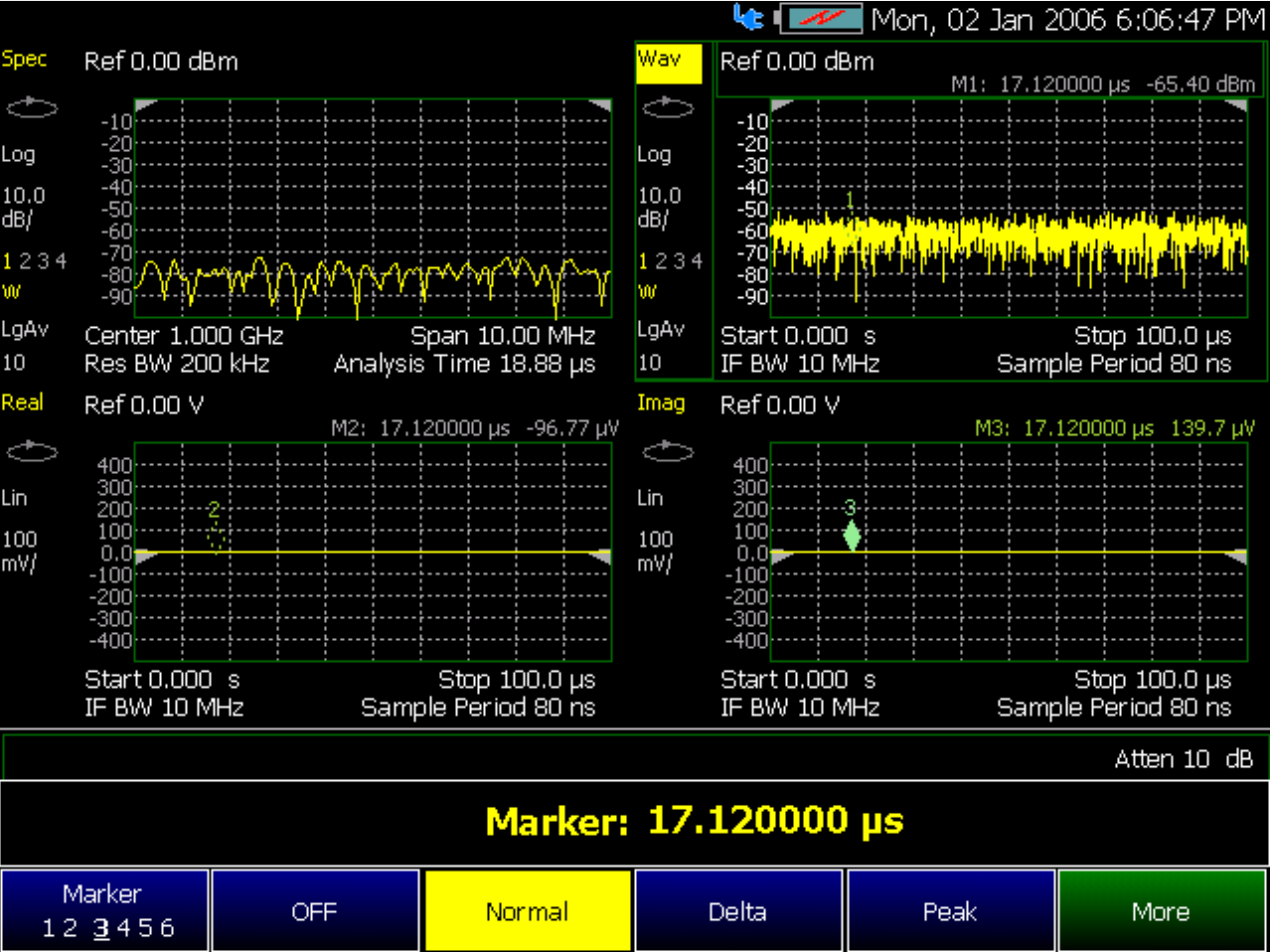
When the Continuous Peak Search marker is on, a peak search is automatically performed for the selected marker after each acquisition. For additional marker functionality, refer to “All about Markers” on page 819.
Summary:
—Cont Peak Search Enables or disables the continuous peak search
—The rules for finding the peak are exactly the same as for Peak Search, including the use of peak criteria rules.
How to measure with the Continuous Peak Search marker
—Press Mkr->/Tools to create or select a Normal or Delta marker to use the Continuous Peak Search marker.
—Then press More (RF Spectrum Only)
—Then press Mkr Properties
—Then Peak Criteria
—Then Cont Peak Search Enables or disables the Continuous peak search marker (default: OFF).
The IQA mode requires all three alignment types: amplitude, RF burst, and channel equalization. Refer to the SA chapter’s “Alignments” on page 219 for information on all alignments.
Trace Display States (IQA Mode)
| If you have Option 351 I/Q Analyzer option, you can directly save your data as MATLAB files (*.mat). Refer to Chapter 11, “IQ Analyzer (IQA) – Option 351”, on page 309 and to Chapter 33, “File Management”, on page 913. If you have the FieldFox’s Remote Server mode (89600 VSA software connectivity), you can use the VSA software to capture and record your data as MATLAB files (*.mat). Learn more about FieldFox and 89600 VSA software, refer to Chapter 18, “Remote Server Mode (Requires SA Option 233)” and to http://helpfiles.keysight.com/csg/89600B/WebHelp/89600.htm. |
—In IQA Mode you can display up to four of the following types of trace states. All IQA settings are applied to all displayed traces. See also “Marker Trace (IQA and SA Mode)” on page 823.
A color-coded legend for displayed traces is visible in the left pane of the SA mode screen:
W = Clear/Write; M = MaxHold; m = MinHold; A = Average; V = View
How to display the Trace States
—Press Trace 6.
—Then Trace 1,2,3,4 repeatedly to select a trace number to display or change its state. Traces are displayed in the following colors:
—Trace 1 – Yellow Trace 2 – Blue
—Trace 3 – Orange Trace 4 – Green
—Then State [current setting]
—Then choose from the following Trace States:
—Clr /Wr (Clear/Write) Displays the actual measured data for each acquisition.
—MaxHold Displays the maximum response of the input signal at each data point over multiple acquisitions. See also Average Count in “Adjusting the Measurement Setup Settings” on page 328.
—MinHold Displays the minimum response of the input signal at each data point over multiple acquisitions. See also Average Count in “Adjusting the Measurement Setup Settings” on page 328.
—Average Each data point is averaged over multiple acquisitions as set by the Average Count setting. Learn more in “Adjusting the Measurement Setup Settings” on page 328.
—View Displays and then holds the last complete measurement trace on the screen. This is similar to storing a trace in memory.
—Blank Displays no trace.
—External Gain - Refer to the SA chapter’s section, “External Gain” on page 166.
—Limit Lines - For information on using Limit Lines, refer to “All about Limit Lines” on page 834.
—Display Lines - For information on using Limit Lines, refer to the SA chapter’s section, “Display Line” on page 226.