9SA (Spectrum Analyzer) Mode (Option 233–Mixed Analyzers)
| To better reflect the enhancements implemented during the alignment process, for firmware versions >A.10.15 “IF Flatness Alignment” is now referred to as “Channel Equalization” or “Channel Equalization Alignment” (ChanEQ Alignment) |
SA mode measures signals at the SA RF IN connector.
SA mode measurements require NO calibration.
For a comprehensive SA mode tutorial, see Spectrum Analysis Basics (Application Note 150) at https://www.keysight.com/us/en/assets/7018-06714/application-notes/5952-0292.pdf
For information on using the FieldFox Remote Viewer which enables you to view the FieldFox from your iOS device, refer to https://www.keysight.com/us/en/assets/7018-04070/application-notes/5991-2938.pd f
Figure 9-1 SA Display with Markers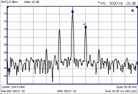
The graphic above shows an SA display with markers.
Carrier with 5 kHz frequency modulation and deviation of 1 kHz.
In this Chapter
See Also
Interference Analyzer: |
Select SA mode before making any setting in this chapter.
Because there is no calibration, these settings can be made in any order.
How to select SA mode
—Press Mode
—Then SA.
The X-axis frequency range determines the frequencies that are measured for each sweep. The default Start frequency is 0 Hz. However, the Start frequency can be set as low as –100 MHz. The internal LO of the FieldFox can be seen at 0 Hz, which will mask signals that may be present.
| Although the start frequency can be set as low as -100 MHz, amplitude accuracy is specified above 9 kHz. Below 9 kHz, frequency accuracy is maintained, but amplitude accuracy is degraded. The FieldFox can be used with both VDI and OML frequency extender. Refer to “Utilities” on page 862, the Configuration Guide at: https://www.keysight.com/us/en/assets/3125-1447/configuration-guides/FieldFox-Handheld-Analyzers-D-models.pdf, and to “Contacting Keysight” on page 5 |
Available ONLY with Opt. 209 and while in Step sweep, SA mode allows reverse sweeps. This means the Start frequency can be higher than the Stop frequency. In addition, the Reverse Swap feature can be used to quickly reverse the Start and Stop frequencies. Learn how in “Reverse Swap” on page 164.
The frequency range of the measurement can be changed using the following methods:
—Set Center and Span frequencies
—Set Start and Stop frequencies
—Toggle between Zero and Last selected span
—Set Full Span of the FieldFox
—Using Channel selection. Learn how in “Channel Selection” on page 162.
—Using Marker > Center (frequency). Learn how in “SA Marker Functions” on page 833.
—Press Freq/Dist.
—Then choose from the following:
—Center and Freq Span frequencies. This is the most common method of entering frequency range. Enter the frequency of interest. The Center frequency is at the exact center of the X-axis. The Frequency Span places half of the frequency range on either side of center. When the Center and Frequency Span values are entered, then the X-axis annotation on the screen shows the Center and Span frequencies. Integration BW (IBW) is coupled to the Frequency Span setting. Frequency Span is 50% wider than the IBW (e.g., if the IBW value is 1 MHz, then the Frequency Span value is 1.5 MHz).
—Start and Stop frequencies. Start is the beginning of the X-axis and Stop is the end of the X-axis. When the Start and Stop frequencies are entered, then the X-axis annotation on the screen shows the Start and Stop frequencies.
—Follow each of these by entering a value using the numeric keypad, the arrows  , or the rotary knob.
—When using the arrows , press Enter. The increment setting of the arrows is based on the current span. This can be changed in SA mode. See “How to change frequency step size” on page 160 below.
—After using the keypad, select a multiplier key. Learn more in “Multiplier Abbreviations” on page 53.
Two more ways to change the frequency range
—Then choose from the following:
—Zero/Last Span Each key press toggles the frequency span between 0 Hz and the last specified frequency span. Learn more about Zero Span in “Zero Span Measurements” on page 204.
—More
—Then Full Span Selects the entire frequency span of the FieldFox. The Center frequency is set automatically.
How to change frequency step size
When using the arrows to change any of the frequency settings, the size of the frequency step can be changed.
—Press Freq/Dist
—Then More
—Then CF Step Auto Manual
—Auto Each press of the arrows increments or decrements the value by 1/10th (one division) of the current frequency span. Note: To change this setting from Manual to Auto, press CF Step twice.
—Manual Type a step size value using the numeric keypad, then select a multiplier key. Learn more in “Multiplier Abbreviations” on page 53.
How to change from Linear to Log Axis View
—Press Freq/Dist > More
—Then choose from the following:
—Log Freq AxisX enables/disables the log frequency X-axis. Disabling the log frequency X-axis, enables the linear frequency X-axis (Default == OFF).
—Full Span Selects the entire frequency span of the FieldFox. The Center frequency is set automatically.
A Radio Standard is a collection of settings that are applied to the FieldFox for specific RF protocols. When a Radio Standard is applied, the FieldFox frequency and channel settings change to that of the standard.
By default, the FieldFox locates the center frequency of the standard in the middle of the screen and sets the frequency span to cover all of the Uplink and Downlink frequencies. The selected Radio Standard name appears in the center of the screen below the X-axis.
After a Radio Standard has been selected, the frequency range can be changed by selecting channel numbers rather than frequency. Learn how in “How to set Frequency Range” on page 159.
When a Channel Measurement is selected such as ACPR, other relevant settings will be changed such as Integration BW. Learn more about Radio Standards and Channel Measurements in “Radio Standards and Channel Measurements” on page 232.
How to select a Radio Standard
—Press Measure 1 OR Freq/Dist then More
—Then Radio Standard
—Then Radio Standard
—Then select a standard using the arrows or rotary knob and press Enter.
Your own custom Radio Standards can be imported into the FieldFox. Custom standards are created in *.csv (spreadsheet) format.
Once imported, the *.csv file is stored in the FieldFox \User Data\ folder. The custom Radio Standards are read and presented at the top of the list of internal Radio Standards.
How to Import and Delete a Custom Radio Standard
First, press Save/Recall and select the Device from which the Radio Standard will be read. Most likely this will be USB or SD Card.
—Press Measure 1 OR Freq/Dist then More
—Then Radio Standard
—Then Radio Standard
—Then Import Radio Standards
—Then select the *.csv file using the arrows or rotary knob and press Enter.
—Custom Radio Standards can be removed from the FieldFox by selecting Measure 1 then Radio Standard then Delete Radio Standard.
—Then select the *.csv file to delete using the arrows or rotary knob and press Enter.
| To overwrite a custom standard that is already uploaded to the FieldFox, you must first delete the *.csv file from the FieldFox, then re-upload the file that contains the standard. A predefined internal standard (such as GSM 450) can NOT be deleted from the FieldFox. |
After a Radio Standard has been selected, the frequency range can be changed by selecting channel numbers rather than frequency. Once enabled, the channel number is appended to the X-axis frequency range.
How to Enable Channel selection
1.Press Freq/Dist > More
2.Then Unit Freq Chan
With Unit == Chan, Channel Direction becomes available and CF Step alters to Channel Step.
How to change the Channel Number of the Measurement
With Unit == Chan the FieldFox will NOT allow you to specify channels outside of the selected Radio Standard.
—Press Freq/Dist
—Then choose from the following:
—Center Channel Places the center frequency of the specified channel in the middle of the X-axis.
—Start Channel Places the lowest frequency of the specified channel at the beginning of the X-axis.
—Stop Channel Places the highest frequency of the specified channel at the end of the X-axis.
—Freq Span Changes the span of frequencies while the center frequency remains unchanged. Integration BW (IBW) is coupled to the Frequency Span setting. Frequency Span is 50% wider than the IBW (e.g., if the IBW value is 1 MHz, then the Frequency Span value is 1.5 MHz).
—Follow each of the above settings by entering a value using the numeric keypad or the rotary knob.
—Use the arrows to increment the channel number by an amount specified by the Channel Step value (see below).
—Then press Enter or Enter.
Select either Uplink or Downlink Frequencies
Press Freq/Dist then More. Press Chan Direction to toggle between Uplink and Downlink. If either of these selections is not available, then the selected Radio Standard does not contain those frequencies. In that case, Chan Direction is grayed out.
Channel number X-axis annotation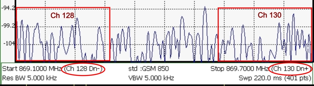
—Dn indicates Downlink channels.
—Up (not shown) indicates Uplink channels
—(−) indicates that the lowest frequency in the channel (128) is at the left edge of the screen.
—(+) indicates that the highest frequency in the channel (130) is at the right edge of the screen.
—When Center Channel or Freq Span is specified, the X-axis shows the Center Freq (Channel) and Frequency Span.
—When Start or Stop Channel is specified, the X-axis shows the Start Freq (Channel) and Stop Freq (Channel).
Change Channel Step Size (Optional)
This setting allows you to use the arrows to increment the channel number by the specified value. The Channel Step softkey appears only when it is valid. Learn how to make it valid in the section, see “How to change the Channel Number of the Measurement” on page 163.
—Press Freq/Dist then More.
—Press Channel Step
—Enter a step value using the numeric keypad, the arrows, or the rotary knob. Then press Enter.
Available ONLY with Opt. 209 and while in Step sweep mode. Each press of the softkey causes the Start and Stop frequencies to swap. The Start becomes the Stop and vice versa. Learn more about Step versus FFT sweeps in “FFT Gating (Opt 238)” on page 210.
—Press Freq/Dist then More.
—Then Reverse Swap
Adjust the Y-axis scale to see the relevant portions of the data trace.
The Y-axis is divided into 10 graticules. A acquisition is shown on the screen as a solid horizontal bar that can be placed at any graticule.
When RF Attenuation set to Auto, the RF Attenuation is coupled to acquisition.
How to set Scale
Press Scale / Amptd. Then choose from the following:
—Autoscale Automatically adjusts the Y-axis to comfortably fit the Minimum and Maximum amplitude of the trace on the screen.
—ScaleEnter a value using the numeric keypad, the Manually adjust the scale per division to view specific areas of the current trace. arrows, or the rotary knob. Then press Enter.
—Ref Level Manually set the value of the reference line. Enter a negative value by pressing Run/Hold (+/-) either before or after typing a value. This can also change the RF Attenuation setting. See “Attenuation Control” on page 167.
—Preamp Refer to “Preamplifier Control (Opt 235)” on page 168.
—RF Atten Refer to “Attenuation Control” on page 167.
—More opens another set of scale softkeys.
Manually set Scale Type, acquisition, and Reference Position.
—Scale Type [current setting]
—Log Logarithmic scale (default setting). The Y-axis reference line represents the specified absolute acquisition in the current Unit selection. Y-axis graticules show dB below or above the reference line.
—Lin Linear scale. The Y-axis reference line represents the specified absolute acquisition in the current Unit selection. Y-axis graticules show percent of acquisition (%) below or above the reference line.
—Unit Refer to “How to Set Y-axis Units” on page 166.
—Corrections Refer to “How to select and edit corrections for Field Strength measurements” on page 169.
—External Gain Refer to “External Gain” on page 166.
—Ref Pos Manually set the position of the reference line. Values must be between 0 (TOP line) and 10 (BOTTOM line). Default position is zero (top).
—PSD Function Enables/disables the Power Spectral Density Function (PSD Function) which is a way to normalize the SA measurement to a 1 Hz Bandwidth. (Default == OFF). Learn more, see “Power Spectral Density (PSD) Function (SA mode Only)” on page 227.
The Unit setting appears for the reference line, marker readouts, and trigger level. All Unit choices are available in both Log and Linear Scale Types.
The UNIT setting survives Mode Preset, but NOT Preset.
—Press Scale / Amptd, then More, then Unit
—Then choose from the following:
— dBm (default setting), dBmV (dB milli Volts), dBµV (dB microVolts), W (watts), V (volts), A (amps), dBmA (dB milliAmps), dBµA (dB microAmps).
“Learn more, refer to “Using the Antenna/Cable Editor” on page 171“.
Antenna correction units are available ONLY by loading or editing an Antenna file that contains the desired units setting. Learn more in “Manage Files” on page 922.
When using an external amplifier or attenuator, the SA mode trace amplitude values can be offset to compensate for the effect of the external device. This effectively moves the reference plane of the SA measurement port out to just beyond the external device. For example, when using an external preamp with gain of +10 dB, enter this value for External Gain, and the data trace across the displayed frequency span will be adjusted down by 10 dB.
When RF Atten is set to Auto, you may see a change in the RF Attenuation value. This is an attempt to measure the signal at top of screen (the acquisition) without overloading the SA first mixer.
How to Set External Gain
1.Press Scale/Amptd.
2.Then More
3.Then External Gain
4.Enter a value using the numeric keypad, the arrows, or the rotary knob (positive for gain; negative for loss). Values less than 5 dB must be typed using the numeric keypad. Then press Enter
ExtGain xx dB is shown at the top of the screen.
Both the RF Attenuation and Preamp functions control the power level into the SA.
When too much power is present at the RF Input port, ADC Over Range appears on the FieldFox screen. This does not necessarily mean that damage has occurred, but that the measurement is probably compressed.
When high power levels are present at the RF Input port, internal attenuation can be switched in to keep the FieldFox receiver from compressing. At extremely high power levels, use external attenuation to protect the internal circuitry from being damaged. Learn more about ADC over range warnings by referring to Chapter 31, “System Settings,” and then to “SA” on page 882
The displayed power level is automatically adjusted for RF Attenuation. As the attenuation value changes, the displayed power level should NOT change.
1.Press Scale/Amptd.
2.Then RF Atten Auto Man.
—Auto RF Attenuation is set by adjusting the acquisition. As the acquisition is lowered, for example from –10 dBm to –30 dBm, the FieldFox assumes that you are looking at low-level signals. The RF Attenuation value is automatically lowered in 5 dB steps to allow low-level signals to be viewed. The RF Attenuation value is never automatically lowered below 5 dB.
—Man RF Attenuation is set manually. The default Attenuation setting is 10 dB. Enter a value between 0 to 30 dB in 5 dB steps using the numeric keypad, the arrows, or the rotary knob. Then press Enter
#Atten xx dB is shown at the top of the screen. (#) means manual setting.
Preamplifier Control (Opt 235)
When very low-level signals are analyzed, an internal preamplifier can be used to boost the signal level by approximately 22 dB. The gain of the preamp is NOT adjustable. The displayed signal level is automatically adjusted for the increase in system gain.
By default, the preamp is OFF.
—Press Scale/Amptd.
—Then Preamp ON OFF The underlined setting is the current setting. When ON, PA is shown to the left of the graticules on the display.
Check for Compressed Measurements
Compression occurs when too much power into an amplifier causes it to no longer amplify in a linear manner. When too much power goes into the FieldFox RF Input connector, the amplifiers in the SA receiver compress and signal power will not be displayed accurately. This can occur even if ADC Over Range is not displayed because devices other than the ADC, such as the mixer, might be compressed. Increase the RF Attenuation value to prevent the SA receiver from being compressed.
How to Check for a Compressed Measurement
1.Using a marker at the signal peak, make note of the signal power level.
2.Increase the RF Attenuation level by 5 dB.
—If the signal level does NOT change, then NO compression exists. This indicates that the signal is in the linear region of the FieldFox receiver.
—If the signal level DOES increase, then the receiver was compressed. Set the RF Attenuation value at the setting when further increases no longer result in an increase in the displayed power level.
To measure the strength of any signal transmitted through the air, an antenna must be connected to the FieldFox. The Field Strength feature allows you to enter the frequency response of the receiving antenna (the Antenna Factor) and associated cabling, and then have amplitude corrections automatically compensate the displayed trace for that response. 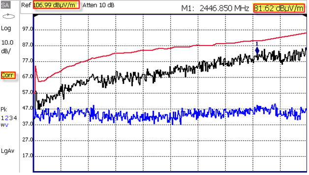
Setting Field Strength Measurements
Trace 1 - Corrected trace with antenna factor. (Antenna == ON, Apply Corr == ON)
Trace 2 - Uncorrected trace (Apply Corr == OFF). The Trace 2 trace state is “View.” For information, refer to “Trace Display States (SA mode)” on page 213
Pink Trace - Current correction factor. See below.
—Learn how to set Y-Axis Units on “How to Set Y-axis Units” on page 166.
—Use a Band Power marker to measure total power over a range of frequencies. Learn how in “Band/Interval Power Marker” on page 229
How to select and edit corrections for Field Strength measurements
The Antenna and Cable correction data survives a Mode Preset and Preset.
All Correction ON/OFF states survive a Mode Preset, but NOT a Preset.
—Press Scale/Amptd > More > Corrections
—Then choose from the following:
— Apply Corrections Auto Disabled Use Auto and Disabled correction for all settings. (Default == Auto).
—Antenna Off – Opens a softkey menu to enable/disable a antenna and edit, save, create a new antenna factors table, recall, and set a storage device location. See also, “How to Use the Antenna and Cable Softkeys” on page 171.
—Cable Off – Opens a softkey menu to enable/disable a cable and edit, save, create a new cable description table, recall, and set a storage device location. See also, “How to Use the Antenna and Cable Softkeys” on page 171.
—More – Opens a softkey menu to View Corrections and set the Amplitude Correction type for your antenna.
Learn more, see “Selecting and Viewing Corrections” on page 170.
—More – Edit/Recall an Antenna file to be used to transmit.
—RcvrSide Antenna Off / On Edit/Recall an Antenna file to be used to receive.
—SrcSide Cable Off / On Edit/Recall a Cable file to be used on the Source side.
—RcvrSide Cable Off / On Edit/Recall a Cable file to be used on the Receiver side.
Selecting and Viewing Corrections
1.Press Scale/Amptd > More > Corrections > More
2.View Corrections ON OFF Turn ON and OFF Pink Trace - Antenna/Cable corrections. This is a composite of all cable/antenna corrections that are currently applied. Available as a useful visual aid, the zero “dB” level (no net correction) is mapped to appear at the -50 dBm on-screen level.
3.Amp Corr Select [Triaxial XYZ] - then choose one of the following:
—Default Receiver side only antenna measurements.
—Src/Rcvr Split to work with non-triaxial receiver and source side antenna measurements.
—Triaxial XYZ (default, when Channel Power is on and when a compatible triaxial antenna’s factors have been imported) for measuring channel measurements and EMF.
4.<Back To return to previous softkey menu.
How to Use the Antenna and Cable Softkeys
The following menu appears when any of the above Antenna Off or Cable Off softkeys are pressed:
—Antenna ON OFF or Cable ON OFF – Turn correction ON or OFF for this Antenna/Cable.
—Edit Antenna or Edit Cable– Edit an Antenna/Cable Correction table. See “Using the Antenna/Cable Editor” on page 171 for more information.
—New – Create a new Antenna/Cable. See Using the Antenna/Cable Editor (below) for more information.
—Save Antenna/Cable – Save the modified Antenna/Cable to a file on the specified Storage Device.
—Recall Antenna/Cable – Read an existing Antenna/Cable file from the specified Storage Device.
—Storage Device – Choose from: Internal, USB, SD. Learn more about these selections in “Set File Type and Select Device” on page 919.
When finished, press Back to return to the previous menu.
Using the Antenna/Cable Editor
The Antenna Editor and the Cable Editor menus are very similar. Both tables include header information, and a Frequency/Value table.
Figure 9-2 FieldFox Antenna Editor– E–Field and H-Field Units Displayed
Figure 9-3 FieldFox Antenna Editors – Settings and Values
How to use the Antenna/Cable Editor
1.Press Scale/Amptd > More > Corrections then choose:
—Antenna Off to open the antenna editing softkeys.
—Cable Off to open the cable editing softkeys.
2.Then Edit Antenna or Edit Cable to open the Antenna / Cable Editor.
3.Press New then Yes to clear all data from the existing Antenna or Cable table and reset header information to default settings.
4.Then use the arrows to select a field.
—To edit header information, press Edit then modify the selected field using the FieldFox labeler.
—Description: Enter a description for the antenna or cable correction table. This is NOT the filename used to save the file.
—Antenna Factor Unit: Determines whether Field Strength measurement Amplitude units will be available or not, and how to convert between them. Select None (default setting) if you just want standard Amplitude units, with a simple dB offset supplied by the correction table. This makes the correction basically identical to a Cable correction. To get Field Strength units, you must choose either dB /m (E-field or dipole antenna), or dB S/m (H-field or loop antenna) to properly identify the Antenna Factors in the table. The scalar measurement Amplitude units (either standard or Field Strength) will then be available at Ampl/more Unit. Learn how in “Scale and Units” on page 165. For details on standard Amplitude units, refer to “How to Set Y-axis Units” on page 166.
—Freq Interpolation: Set to LINear by the FieldFox and can NOT be edited.
—To edit Frequency/Value pairs, enter numbers using the numeric keypad, and a frequency suffix when necessary.
—For both Cable Loss and Antenna Factor values, Positive numbers indicate loss (we need ADD something positive to compensate for it), and Negative is indicative of some existing gain.
—Antenna Factor describes the dB value needed to accurately display a far-field signal in terms that are in the units listed below. When the antenna has low gain, or low efficiency, the dB value to be added is larger.
—Antenna Factor Unit sets the type of antenna factor unit used in your measurement (i.e., dB /m or dB S/m).
—When one Freq/Value pair is entered, that correction value is applied to the entire displayed frequency span.
—When two or more Freq/Value pairs are entered, the data points between the lowest and highest frequencies are corrected. Linear interpolation is applied between frequencies when necessary.
5.Optionally choose from the following:
—Previous / Next Page Quickly scrolls through pages of Freq/Value data.
—Add Row Add a blank Freq/Value pair to the table,
—Delete/Clear then:
—Delete Row Remove the selected Freq/Value pair from the table.
—Clear All then Yes Remove all Freq/Value pairs from the table and resets header information to default settings.
When the table edits are complete
1.Press Done to close the Antenna/Cable Editor.
2.PressAntenna Off On > On.
Then choose your final measurement amplitude unit, under Scale/more. If you selected either dB /m or dB S/m for the Antenna Factor unit, you should see this list of available Field Strength units
3.Press Scale/Amptd > More > Unit dBµV/m and choose from:
—dBµV/m == dB micro Volts per meter
—dBm/m^2 == dBm per meter squared
—V/m == volts per meter
—W/cm^2 == watts per cm squared
—W/m^2 == watts per meter squared
—dBµA/m == dB micro Amps per meter
—dBG == dB gauss
—dBpT == dB pico tesla
4.Press Back > Back > Save Antenna or Save Cable to save your changes to the specified Storage Device. Enter a filename using the FieldFox labeler (learn more in “How to use the FieldFox labeler ” on page 916). Learn more about Antenna and Cable files below.
Optional:
—Press Recall Antenna or Recall Cable to load an Antenna or Cable file from the specified Storage Device.
—Storage Device Changes the device used to save or recall files. Choose from Internal (default setting), USB (must be connected) or SD card. This is a different setting from the Save/Recall Storage Device setting.
About Antenna and Cable files
—Cable files are saved and recalled from the Cables folder.
—Antenna files are saved and recalled from the Antenna folder.
—To DELETE Cable or Antenna files, use the Manage Files feature. Learn more in “Manage Files” on page 922.
—If the folder does not already exist on a USB or SD card, it is created automatically before storing the file.
—All Antenna and Cable files are saved and recalled as *.csv files, which allows them to also be read by spreadsheet programs.
—The FieldFox can also read *.ANT (Antenna) files that were created from older Keysight Spectrum Analyzers.
—Cable and Antenna (*.csv or *.ANT) files canNOT be edited in Data Link software.
How to create a Cable file from an S21 (NA mode) or an Insertion Loss (CAT mode) measurement
1.Measure the S21 or Insertion Loss of a cable. In NA mode, select either LogMag, Linear, or VSWR formats.
2.Use Manage Folders to change the active folder to CABLES. Learn how in “Manage Files” on page 922.
3.While in NA mode, save the measurement as a *.csv file. Learn how in “How to Save a File” on page 914.
4.In Channel Scanner or SA mode, select Corrections, then recall the *.csv file for correction.
Source Tracking Offset and Offset Reversal
—N991xD/5xD FieldFox Combination Analyzers to have Options 210, and 233
—N993xD/6xD Spectrum Analyzers to have Options 220
Source offset tracking is used to offset the Source frequency from the Receiver frequency by a fixed offset at every tune frequency. This feature is used when the DUT contains a frequency translation device or mixer.
How to set Tracking Offset and Offset Reversal
1.On the Receiver unit, press Measure 1 > Source > Advanced
2.Then choose one or both of the following:
—Tracking Offset Enter an offset value (Default == OFF).
—OffsetReversal Determines whether Receiver Freq is added to or subtracted from the Offset Freq.
—OFF SourceFreq = Offset + RecFreq. Use to measure Upconverters.
—ON SourceFreq = Offset - RecFreq. Use to measure Downconverters. The source sweeps in Reverse direction. Note: The Offset Freq. MUST be larger than the Receiver Stop Freq.
The Tune & Listen feature can be used to identify an interfering AM or FM signal.
The demodulated AM or FM signal can be heard through the internal speaker or through headphones using the 3.5 mm jack located on the FieldFox side panel.
The Tune & Listen tuner is separate from the SA display. This allows you to listen to one frequency while displaying a different range of frequencies. The Tune & Listen measurement alternates between normal SA sweeps for the display and performing audio demodulation at the Tune Frequency. See the Listen Time setting for more information.
Figure 9-4 Tune & Listen ON
In the graphic above, Tune & Listen ON with Tune Frequency is indicated by a vertical bar (highlighted). This section contains the following:
How to select Tune & Listen
—Press Measure 1 > Analog Demod Tune & Listen > Tune & Listen
—Then choose a demodulation type. Select a setting based on the type of interfering signal you suspect is being broadcast.
Press Meas Setup 4 > Tnl Demod Type then
—AM – Sets AM (Double-sideband with carrier) as the modulation type.
—FM Narrow – Sets Frequency Modulation; Narrow bandwidth. Choose when interfering transmission consist of voice or data.
—FM Wide – Sets Frequency Modulation; Narrow bandwidth. Choose when interfering transmission consist of voice or data.
—AM USB – Sets the modulation type to AM upper sideband. Annotation: AM USB @ Center Frequency displayed at the top of display. See also, “TnL AM SSB Gain”.
—AM LSB – Sets the modulation type to AM lower sideband. Annotation: AM LSB @ Center Frequency displayed at the top of display. See also, “TnL AM SSB Gain”.
See also, “How to select Analog Demod (Metrics)” on page 182.
When you select AM USB or AM LSB softkeys, the TnL AM SSB Gain softkey becomes active.
—Press Meas Setup 4 > More then
—TnL AM SSB Gain – sets the gain in the IF path for TnL SSB measurements (the optimal IF path gain is automatically determined/set for regular AM and all the other demod types, but it cannot be automatically determined for AM SSB so it has to set it manually).
The goal is to set the gain as high as possible (to take advantage of the range of the IF and audio paths) without distorting the audio signal. It is recommended that you keep increasing the gain until you hear distortion in the audio and then back off until you no longer hear any distortion. The system volume setting should still be used to determine the final desired volume/level of the audio output. Learn more, see also Chapter 31, “System Settings.” and “Audio (Volume) Control” on page 859.
(Default == 0, Minimum == –50 dB, Maximum == +50 dB)
The Tune & Listen tuner is separate from the SA display. This allows you to listen to one frequency while displaying a different range of frequencies.
Set the Tune Frequency using one of three methods:
1.Selecting Preset > Mode Preset, sets Tune Frequency to 3.25 GHz.
2.Specify Tune Frequency:
a.Press Meas Setup 4 > Tune Freq
b.Enter a value using the numeric keypad, arrows, or the rotary knob. Then select a multiplier key. Learn about multiplier abbreviations “Multiplier Abbreviations” on page 53.
3.Using Mkr->Tune Freq:
—Create a normal marker at the frequency of interest. Learn how in “How to create Markers” on page 819.
a.Press Mkr->/Tools
b.Then Mkr->TuneFreq to change the Tune Frequency to that of the marker.
| To improve sound quality, try increasing power by reducing the Attenuation setting and, if available, turn ON the Preamplifier. Learn how in “Attenuation Control” on page 167 |
While Tune & Listen is actively demodulating a signal, the SA does not sweep and update the display. Listen Time sets the amount of time that the FieldFox demodulates, then stops to perform a single sweep and update the display, then again demodulates.
—Press Meas Setup 4 > Listen Time
—Enter a value using the numeric keypad, arrows, or the rotary knob. Then select a multiplier key. Learn about multiplier abbreviations.
To increase or decrease the Volume of the demodulated signal:
—Press Meas Setup 4 > Volume
—Enter a value in percent between 0 and 100 (loudest) using the numeric keypad, arrows, or the rotary knob.
—Volume can also be changed and easily muted from the System menu. Learn more in “How to set the FieldFox Volume Control” on page 859.
To quickly stop the audio demodulation and perform only the normal SA sweeps, select the following:
—Press Meas Setup 4 > Audio Demod ON OFF > OFF
Setting the Marker Counter Precision Softkey
When AM Tune & Listen, FM (narrow) Tune & Listen, or FM (wide) Tune & Listen are selected, you can choose from the following:
—Press Marker > Peak
—Press Mkr->/Tools > More > Mkr Properties > Counter Precision – Sets the AM or FM Metric demodulated signal’s marker precision (.1 Hz, 1 Hz, 10 Hz; Default == 0.1 Hz).
The Counter Precision softkey is not available when AM Metric or FM Metric are enabled. See also, “Setting the Mkr->TuneFreq Softkey” on page 180.
Setting the Mkr->TuneFreq Softkey
When AM Tune & Listen, FM (narrow) Tune & Listen, or FM (wide) Tune & Listen are selected, you can choose from the following:
—Press Marker > Normal
—Press Mkr->/Tools > Mkr->TuneFreq – The Tune & Listen Frequency becomes the frequency of the active marker (When AM Metrics or FM Metrics are selected this softkey is inactive).
See also, “How to use Marker Functions” on page 832.

The Tune & Listen feature can be used to identify an interfering AM or FM signal. Also, AM/FM Metrics displays the demodulated signal and the audio frequency spectrum.
The demodulated AM or FM signal can be heard through the internal speaker or through headphones using the 3.5 mm jack located on the FieldFox side panel.
The Analog Demod spectrum is displayed alongside the SA displayed trace. This enables you to listen and display a carrier frequency and it’s harmonics. The Analog Demod measurement displays a normal SA sweeps for the display while performing audio demodulation at the carrier Frequency. See the “How to select Analog Demod (Metrics)” on page 182 setting for more information.
Figure 9-5 AM DSB (Metrics) – Demodulation Spectrum
In the graphic above, Analog Demod ON and Demod Metrics is indicated above in the x2 displays of carrier spectrum content. For this example, AM Modulation Metrics are displayed in the lower half of the display. See also, Figure 9-6 on page 189, Figure 9-7 on page 189, Figure 9-8 on page 190, and Figure 9-9 on page 190.
How to select Analog Demod (Metrics)
Analog demodulation can demodulate AM DSB, AM SSB, FM, FM Stereo / RDS, PM signals. Under analog demodulation metrics the following information is reported for each signal type: Carrier power, modulation rate, SINAD, THD, plus deviation, depth, or RMS depending on the signal. Metrics also displays the demodulated signal and the audio frequency spectrum.
Learn more, Chapter 27, “AM/FM Metrics (Option 355).”
—Press Measure 1 > Analog Demod Tune & Listen > Analog Demodulation
—Demod Type – Then choose a demodulation metric type. Select a setting based on the type of interfering signal you suspect is being broadcast. IMPORTANT! The FieldFox contains only one speaker that supports mono audio output (i.e., if you play a stereo WAVE file, the Left and Right channels are output in mono audio). If you want to output a stereo WAVE file in stereo (to hear the left and right channels separately on the FieldFox) you have to use the headphone jack and stereo headphones (i.e., most earbuds, headphones, etcetera support stereo). Learn more, see also Chapter 31, “System Settings.” and “Audio (Volume) Control” on page 859.
—AM – AM (double sideband). Displayed values for AM Modulation (metrics) – (i.e., includes AM Mod Depth, AM Demod Waveform, SINAD, THD, Carrier Power, Carrier Freq, Modulation rate).
—AM SSB – AM single sideband. Displayed values for AM SSB (metrics) – (i.e., includes SSB RMS Level, SSD Demod Waveform, SINAD, THD, RF Power, Modulation rate).
—FM – Displayed values for FM Modulation (metrics) (i.e., includes Freq Deviation, FM Demod Waveform (Time)/Spectrum (Frequency), Carrier Power, Carrier Freq, Modulation Rate, SINAD, THD).
—FM Stereo / RDS – Displayed values for FM Stereo / RDS (Radio Design System); (Metrics) – (i.e., includes Freq Deviation, FM Demod Waveform (Time)/Spectrum (Frequency), Carrier Power, Carrier Freq, Modulation Rate, SINAD, THD, Dist/ Total VRMS). When FM Stereo /RDS is selected as the demodulation type, a Warning message is displayed for a few seconds at the start of the sweep; the sweep is 30 to 50 seconds long. The message reads: "Warning: Slow Measurement. RDS Measurement in Progress."
—PM – Displayed values for PM Modulation Metrics (i.e., includes PM Deviation, PM Demod Waveform, SINAD, THD, Carrier Power, Carrier Freq, Modulation Rate).
—Tune & Listen OFF – Opens a menu of Tune & Listen demod softkeys. Tune & Listen can be set when you are in Analog Demodulation mode, so you can enable Tune & Listen sweeps in between your Analog Demod sweeps. To learn more about the Tune & Listen softkey menu choices, refer to “Tune & Listen (AM/FM)” on page 176.
See also, “How to make Analog Demodulation (Metrics) Settings” on page 183.
How to make Analog Demodulation (Metrics) Settings
The following softkeys are available when one of the Analog Demodulation metrics measurements is pressed. See also, “How to select Tune & Listen” on page 177.
If AM DSB, choose from:
—AM Top Y – Determines the Y axis percentage (0% to ±100%) of the AM demodulation waveform is displayed (Default == 100%).
If AM SSB, choose from:
—SSB Top Y – Determines the Y axis voltage (0 nV to ±100mV) of the AM SSB demodulation waveform is displayed (Default == 100 mV).
If FM, choose from:
—FM Top Y – Determines the Y axis frequency (1 kHz to 1 GHz) of the FM demodulation waveform is displayed (Default == 100 kHz).
If FM Stereo / RDS, choose from:
—FM Top Y – Determines the Y axis frequency (1 kHz to 1 GHz) of the FM demodulation waveform is displayed (Default == 100 kHz).
If PM, choose from:
—PM Top Y – Determines the Y axis phase (0 to 100 radians) of the PM demodulation waveform is displayed (Default == 5).
For any of the following: AM DSB, AM SSB, FM, FM Stereo / RDS, or PM, choose from:
Refer to Figure 9-6 on page 189, Figure 9-7 on page 189, Figure 9-8 on page 190, and Figure 9-9 on page 190.
—Demod SwpT – Sets the X-axis to display the demodulation sweep time for the demodulated waveform (minimum == 50 μs; maximum == 50 ms).
—Peak OFF ON – This adds peak positive and peak negative metrics to the main metrics measurement. For example, in FM peak ON will include peak positive (Peak +) and negative (Peak -) frequency deviation metrics to appear. Peak ON will also enable peak traces on the demodulation waveform and audio frequency spectrum (Default == OFF).
—Demod Type – Sets the demodulation type.
Choose from AM, AM SSB, FM, FM Stereo / RDS, and PM.
—Then, press More – opens a menu of softkeys: Average Type, Average Count, and Demod View Time Freq.
—Average Type – Selects the way the demodulated signal values are averaged. Choices are Power (#PAvg annotation is displayed), Log (#LgAv annotation is displayed), Voltage (#VAvg annotation is displayed). Auto is the default and when selected the FieldFox chooses the type of averaging that is used based on the current settings.
—Average Count – Determines the amount of averaging used (1 to 10K; Default == 10).
—Demod Filters – Refer to “How to Set the Demod Filters” on page 186.
—Demod View Time Freq – Toggles how the demodulated signals are displayed (Time (waveform) or Frequency (spectrum)); Default == Time).
—Audio Capture Playback – Refer to “Setting the Audio Capture Playback Softkeys” on page 185.
Setting the Alternate Frequency (AF) Freq/Dist Softkeys
When AM DSB, AM SSB, FM, FM Stereo / RDS, or PM are selected and Demod View == Freq, you can choose from the following:
—Press Freq/Dist then choose:
—AF Start Freq – Sets the AF start frequency for the AM or FM demodulated signal.
—AF Stop Freq – Sets the AF stop frequency for the AM or FM demodulated signal.
—AF Full Span – Sets the AF full span frequency for the AM or FM demodulated signal.
Also, you can set the standard Center, Freq Span, and other frequency softkeys.
Setting the Alternate Frequency (AF) RBW Softkey
When AM DSB, AM SSB, FM, FM Stereo / RDS, or PM are selected and Demod View == Freq, you can choose from the following:
—Press BW 2 then choose:
—AF RBW – Sets the audio frequency (AF) resolution BW for the AM or FM demodulated signal (Manual or Auto; Default == Auto).
Setting the Audio Capture Playback Softkeys
The FieldFox analog demodulation audio capture playback feature allows you to capture/record the demodulated audio associated with an analog demodulation measurement (AM DSB, AM SSB, FM, FM Stereo or PM) and save it as an audio file. It also allows you to recall and playback audio files through FieldFox's built-in speaker or headphones. Currently, the audio capture playback feature supports WAVE files with mono or stereo LPCM data sampled at 48,000 Hz with 16 bits per sample. If you are unable to hear your audio data files (*.wav), verify that your System > Preferences > Preferences > Audio is set to On.
When Analog Demod is selected, you can choose from the following:
—Press Meas Setup 4 > More > Audio Capture Playback then
—If you want to initiate an audio capture:
Press Capture
—If you want to stop an audio capture:
Press Stop to stop the current capture of audio data and depending on the timing of pressing Stop, possibly prevent the audio data from being stored.
—If you have previously stored an audio file:
Press Playback then
—Play – to play the last current audio file (*.wave) loaded into memory.
—Stop – to disable playback of the current audio file.
—Volume Mute – to enable disable volume and to adjust the volume from 0 to 100 (Default == Mute /Volume == 10).
—Load Audio File – to load a previously stored audio (.wave) file.
—Cap Auto–Load – enable/disables automatically loading of a captured audio (.wav) file (Default == OFF).
—Press Capture Settings then
—Capture Count – sets the number of audio captures for a measurement (Default ==1; Settable: 1 to 100K).
—Capture Time – sets the capture time (Default == 100 ms). Minimum/Maximum capture times vary with other settings.
—Stereo Channel – When Demod Type == FM Stereo / RDS, this softkey sets the type of audio to be captured and stored: (Choose single channel: Mono (L+R), Left (L), Right (R), and Difference (L–R). Or choose two channel: Stereo (L&R). Default == Mono (L+R).
Then Choose:
Mono (L+R) | Sets the audio recording to Mono (single channel) and combining left and right speaker sounds. This is the default. |
Stereo (L&R) | Sets the audio recorded to be stereo (two channels). |
Left (L) | Sets the audio to be recorded to be the left speaker only. |
Right (R) | Sets the audio to be recorded to be the right speaker only. |
Difference (L–R) | Sets the audio to be recorded to be the value of the left side minus the right side of the audio data (single channel). |
—Press Back to return to previous menu.
—Then File Settings then
—Filename – Opens the filename labeler to specify a filename.
—Timestamp OFF ON – Enables/disables a timestamp label on your audio (.wav) filename.
—Storage Device – Sets the storage device location for your audio (.wav) file. Select Internal (default), SD Card, or USB.
For more on file settings refer to Chapter 33, “File Management.”
The demodulation (Demod) filters and de-emphasis options help you accurately recover and analyze the modulating signal. The demod filters apply to all demod types (AM DSB, AM SSB, FM, FM Stereo and PM), while the de-emphasis options only apply to the FM and FM stereo demod types.
—Press Meas Setup 4 > Demod Filters then
—Lowpass Filter None – then choose:
None | No lowpass filter is selected. |
300 Hz | 5-Pole Butterworth LPF with 3 dB cutoff frequency of 300 Hz. |
3 kHz | 5-Pole Butterworth LPF with 3 dB cutoff frequency of 3 kHz. |
15 kHz | 5-Pole Butterworth LPF with 3 dB cutoff frequency of 15 kHz. |
30 kHz | 3-Pole Butterworth LPF with 3 dB cutoff frequency of 30 kHz. |
80 kHz | 3-Pole Butterworth LPF with 3 dB cutoff frequency of 80 kHz. |
100 kHz | 3-Pole Butterworth LPF with 3 dB cutoff frequency of 100 kHz. |
20 kHz | 9-Pole Bessel LPF with 3 dB cutoff frequency of 20 kHz. |
300 kHz | 3-Pole Butterworth LPF with 3 dB cutoff frequency of 300 kHz. |
Custom | 5-Pole Butterworth LPF with a custom 3 dB cutoff frequency (determined by the LPF 3 dB Cutoff setting). |
—LPF 3 dB Cutoff 300.000 Hz – When the Lowpass filter is set to Custom, sets the customized LPF 3 dB cutoff frequency for the lowpass filter (Default == 300 Hz; Minimum == 90 Hz, Maximum == 5 MHz).
—Highpass Filter None – then choose:
None | No highpass filter is selected. |
20 Hz | 2-Pole Butterworth HPF with 3 dB cutoff frequency of 20 Hz. |
50 Hz | 2-Pole Butterworth HPF with 3 dB cutoff frequency of 50 Hz. |
300 Hz | 2-Pole Butterworth HPF with 3 dB cutoff frequency of 300 Hz. |
400 Hz | 10-Pole Butterworth HPF with 3 dB cutoff frequency of 400 Hz. |
Custom | 5-Pole Butterworth HPF with a custom 3 dB cutoff frequency (determined by the HPF 3 dB Cutoff setting). |
—HPF 3 dB Cutoff 500.000 Hz – When the Highpass Filter is set to Custom, sets the customized HPF 3 dB cutoff frequency for the highpass filter (Default == 500 Hz; Minimum == 20 Hz, Maximum == Varies, depending on the AF Span).
—Bandpass Filter None – Sets the Bandpass Filter for the current measurement (Choices: None, CCITT, A-Weighted, C-Weighted, C-Message, CCIR-1k Weighted, CCIR-2k Weighted, or CCIR Unweighted). Default == None.
—More – FM and FM Stereo only. Opens a softkey menu to enable/disable the De-Emphasis softkeys.
——De-Emphasis OFF ON – Enables/disables the de-emphasis applied to the demodulated signal.
——De-Emphasis T – Sets the amount of de-emphasis applied to the demodulated signal.
Setting the Marker Counter Gate Softkey
When AM Metric or FM Metric are selected, you can choose from the following:
—Press Marker > Peak
—Press Mkr->/Tools > More > Mkr Properties > Counter Gate – Sets the AM or FM Tune & Listen demodulated signal’s counter window time (Minimum == 1 ms and Maximum == 2s; Default == 100 ms).
The Counter Gate softkey is not available when AM Tune & Listen, FM (narrow) Tune & Listen, or FM (wide) Tune & Listen are enabled. Refer to Figure 9-9 on page 190.
See also, “How to use Marker Functions” on page 832.
Figure 9-6 AM DSB (Metrics) – Demodulation Waveform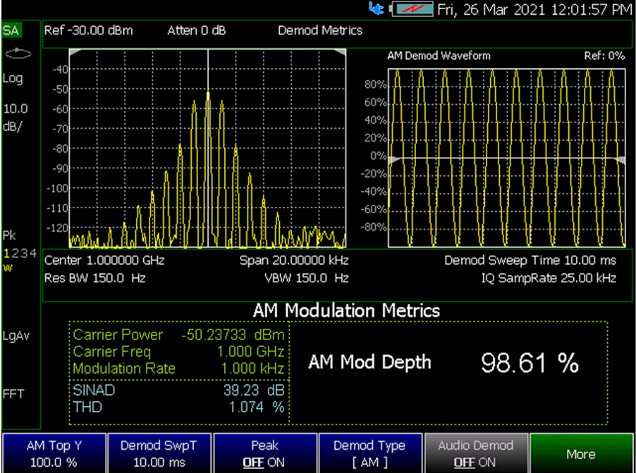
Figure 9-7 FM Metrics – Demodulation Spectrum
Figure 9-8 FM (Metrics) – Demodulation Waveform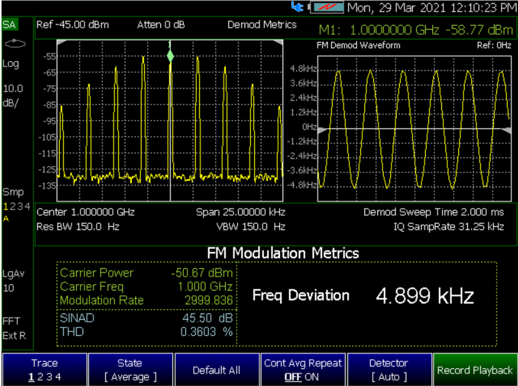
Figure 9-9 FM (Metrics) - Counter Gate and FM Demodulation Waveform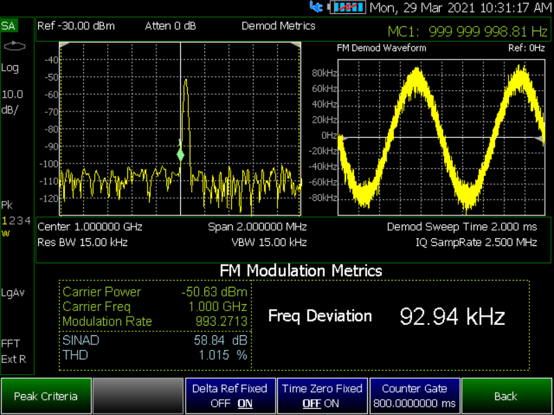
Figure 9-10 Audio Capture with Annotation Examples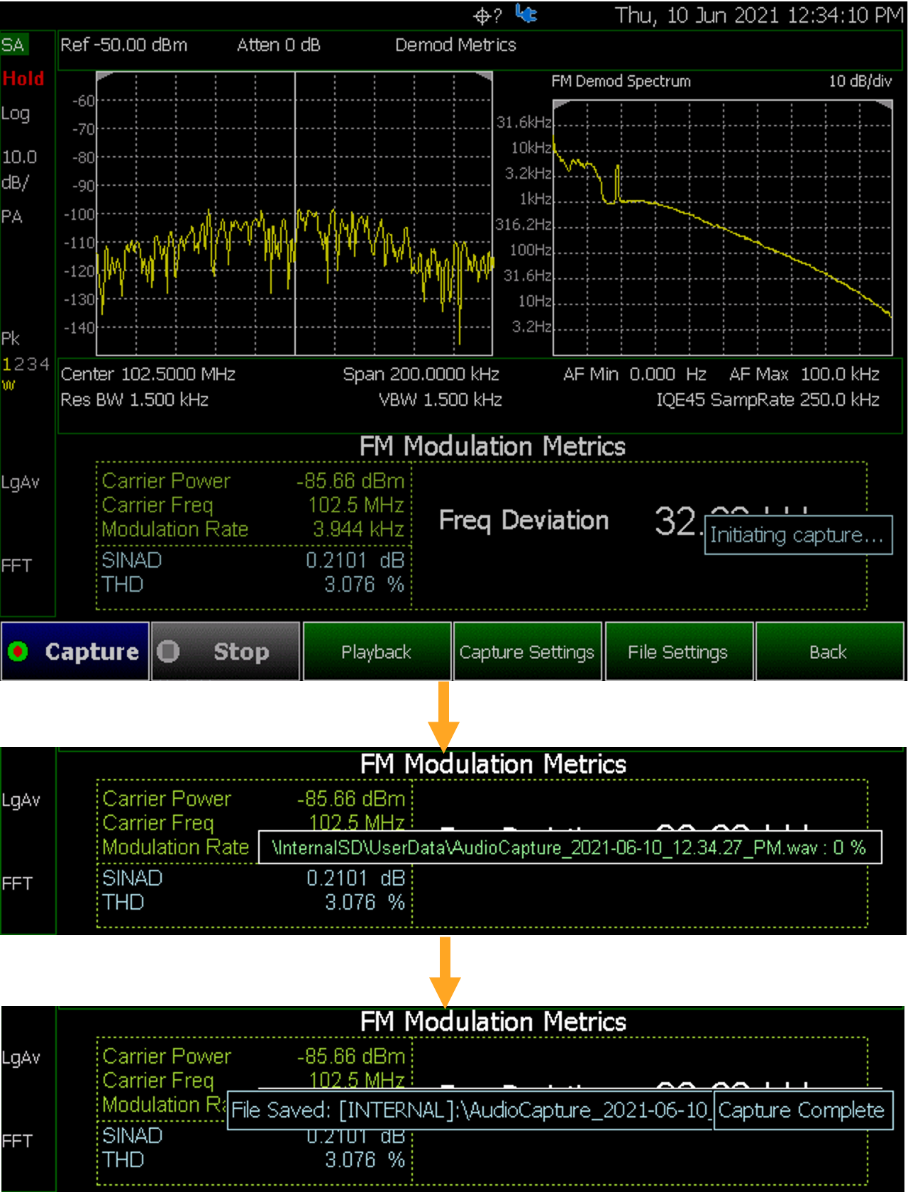
Independent Source/Tracking Generator
For best results, when using the independent source feature, all alignment and the battery saver features should be turned off. Refer to “All Alignment and Align All Now” on page 222 and “Preferences” on page 870 |
This feature may require an option. For a comprehensive list, view the FieldFox Configuration Guide at: https://www.keysight.com/us/en/assets/3125-1447/configuration-guides/FieldFox-Handheld-Analyzers-D-models.pdf.
A tracking generator, a popular option with Spectrum Analyzers, is a source which always tracks the SA receiver.
Like a traditional tracking generator, the Independent Source feature can set the internal FieldFox source to track the SA receiver frequency range. It can also set the internal source to a CW frequency that is independent of the SA frequency.
To view the internal source, you must connect a cable or device between the RF Output connector and the RF Input connector.
How to make Independent Source Settings
—Press Measure 1 > Source
—Source Enable ON OFF
—ON Turns ON the internal source.
—OFF Turns OFF the internal source.
—Source Tracking Choose from the following:
—Sweep The internal source frequency can track the SA receiver. Center frequency Src is annotated on the screen
Sweep softkey is only available if the SA is licensed with Tracking Generator capability (Option 220 for SA only model or Option 210 for combo boxes VNA/NA model). Refer to Figure 9-12 on page 194. |
—OFF The source is set to a CW frequency independent from the SA settings. Srcw is annotated on the screen.
—Center Freq The source is set to a CW frequency, but that frequency “tracks” the SA receiver Center Frequency settings. Therefore, the signal always appears at center of the display. Srcp is annotated on the screen.
—Pulse Gen Only available for B/C model equipped with Pulse Generator license (Option 357) and operating in SA mode. SrcPg is annotated on the screen. Refer to “Track the Pulse Generator ” on page 195.
—Source Power Sets the source power level. Choose from:
—Leveled Enter a value from –60 dBm to 10 dBm using the numeric keypad, arrows, or the rotary knob1. The source power is reasonably flat across the frequency span.
—MAX The power level is set to the maximum achievable power level at each frequency. This results in the power level NOT being flat across the frequency span.
—Source CW Freq Sets the CW frequency that is used.
When Source Enable is ON, Source CW Freq softkey is enabled ONLY when Source Tracking is set to OFF. |
—Advance Only activated exclusively with the Sweep Tracking license (TG capability). Choose one or both of the following:
—Tracking Offset Enter an offset value using the numeric keypad, arrows, or the rotary knob1. The offset value range is +/- maximum frequency of the model.
—OfsTrk Reversal Determines whether Receiver Freq is added to or subtracted from the Offset Freq.
——OFF SourceFreq = Offset + RecFreq. Use to measure Upconverters1.
——ON SourceFreq = Offset - RecFreq. Use to measure Downconverters1. The source sweeps in Reverse direction.
For the OfsTrk Reversal ON, the Offset Frequency MUST be larger than the Receiver Stop Frequency. |
The Independent Source output signal may be momentarily interrupted for automatic SA Receiver alignments or Battery Saver functionality. |
To prevent automatic alignments from interrupting the source, turn off all alignment. Refer to “All Alignment and Align All Now” on page 222.
—Press Cal 5
—Then press All Alignment
—Then press OFF or Hold to disable All Alignment
To prevent Battery Saver from interrupting the source, turned off Battery Saver. Learn more in “Battery Saver” on page 873.
—Press System 7 > Preferences > Preferences
—Then in the table, select Battery Saver value column and press Edit
—Then press Battery Saver to toggle OFF to disable Battery Saver
—Then press Done Edit to commit the edit
Figure 9-11 Source Tracking Softkey Menu in SA mode without Tracking Generator Capability
Figure 9-12 Source Tracking Softkey Menu in SA mode with Tracking Generator Capability
This feature required Pulse Generator license (Option 357), allows the Independent Source mode to effectively retain the settings from the most recent activity, specifically when the Pulse Generator mode was last used with RF enabled.
To utilize this feature, users should navigate to the Pulse Generator, configure a signal and ensure that RF is set to ON. Learn more in Chapter 24, “Pulse Generator Mode – Option 357”, on page 653
How to make Pulse Generator Tracking Settings
—Press Measure 1 > Source > Source Tracking
—Then press Pulse Gen Only available for B/C model equipped with Pulse Generator license (Option 357) and operating in SA mode. Track the pulse generator signal to replicate the same signal setup established in Pulse Generator mode. SrcPg is annotated on the screen.
Pulse Gen softkey appears greyed out and cannot be selected despite having Option 357 on B/C model. Refer to Figure 9-13 on page 195. This occurs because the signal has not been configured with RF ON within the Pulse Generator mode. Learn more in Chapter 24, “Pulse Generator Mode – Option 357”, on page 653. |
When Source Tracking is set to Pulse Gen, Source Power and Source CW Freq are disabled and cannot be adjusted. The Source CW Freq reveals the RF Freq relayed from the Pulse Generator mode. Refer to Figure 9-14 on page 195 and Figure 9-15 on page 196 for track the Pulse Gen example. |
Figure 9-13 Softkey Menu: Pulse Generator Not Configured (RF OFF) - Pulse Gen Greyed out
Figure 9-14 Softkey Menu: Pulse Generator Configured (RF ON) - Pulse Gen Enabled
Figure 9-15 Track the Pulse Gen in SA mode Example - FM Sine Modulated Signal Setup Using Pulse Generator Mode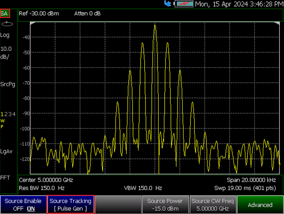
Resolution Bandwidth (Res BW)
In SA mode, the Res BW provides the ability to resolve, or see closely spaced signals. The narrower (lower) the Res BW, the better the spectrum analyzer can resolve signals. In addition, as the Res BW is narrowed, less noise is measured by the spectrum analyzer ADC and the noise floor on the display lowers as a result. This allows low level signals to be seen and measured. However, as the Res BW is narrowed, the sweep speed becomes slower. See “Very Long Sweep Times” on page 204.
1.Press BW 2 > Res BW.
2.Then choose from the following:
—Auto Res BW is coupled to the frequency span. As the frequency span is narrowed, the Res BW is also narrowed providing increased ability to resolve signals.
To change this setting from Man to Auto, press Res BW twice.
—Man Enter a Res BW value using the numeric keypad, the arrows, or the rotary knob. Then press a multiplier if necessary or press Enter
The current Res BW setting is shown at the bottom of the screen.
#Res BW x.xx XHz (#) means manual setting.
This setting could impact the accuracy of the measurement. See Specifications in Appendix B.
| The Res BW setting also affects the Sweep Type setting. Learn how in “Sweep Type” on page 198. |
Video Bandwidth (Video BW)
Video BW is a smoothing operation that is performed after measurement data is acquired. The trace data is effectively smoothed so that the average power level of the displayed noise is the same, but the peaks and valleys of adjacent data points are smoothed together. More smoothing occurs as the Video BW is set lower. However, as the Video BW is narrowed, the sweep speed becomes slower.
1.Press BW 2.
2.Then Video BW
3.Then choose from the following:
—Auto Couples Video BW to the ResBW in a 1-to-1 ratio.
—Man Enter a Video BW value using the numeric keypad, the arrows, or the rotary knob. Then press a multiplier if necessary or press Enter. Setting VBW higher than RBW may smooth the trace.
| To change this setting from Man to Auto, press Video BW twice. |
The current Video BW setting is shown at the bottom of the screen.
# VBW x.xx XHz (#) means manual setting.
When the Res BW/Video BW ratio exceeds 10,000, a Meas UNCAL warning may appear to indicate that the Video BW filter has reached the maximum capacity for averaging.
AF RBW (Audio-Frequency Resolution BW)
AF RBW - sets the audio-frequency resolution bandwidth for the selected frequency (Default == Auto).
1.Press BW 2 > AF RBW
2.Then choose from the following:
—Auto Couples AF BW to the Resolution BW in a 1-to-1 ratio.
—Man Enter a AF BW value using the numeric keypad, the arrows, or the rotary knob. Then press a multiplier if necessary or press Enter. Setting AF BW higher than RBW may smooth the trace.
| To change this setting from Man to Auto, press AF RBW twice. |
The current AF RBW setting is shown at the bottom of the screen.
# AF RBW x.xx XHz (#) means manual setting.
When the Res BW/AF RBW ratio exceeds 10,000, a Meas UNCAL warning may appear to indicate that the AF RBW filter has reached the maximum capacity for averaging.
In SA mode, the FieldFox uses two sweep types to process inputs signals. The sweep type that is currently being used (FFT or Step) is displayed in the lower-left corner of the FieldFox screen.
For a more comprehensive tutorial, see Spectrum Analysis Basics (App Note 150) at https://www.keysight.com/us/en/assets/7018-06714/application-notes/5952-0292.pdf
1.Press BW 2 > Advanced > Sweep Type
2.Then choose from the following:
—Auto The FieldFox selects the most efficient sweep type based on the Res BW. When Res BW is set to 200 kHz and below, FFT sweep type is selected. Above 200 kHz, Step sweep type is being performed.
—FFT The FieldFox uses FFT sweep type regardless of the Res BW.
—Step The FieldFox uses Step sweep type regardless of the Res BW. This is useful for capturing impulsive noise that may be generated from nearby electrical equipment.
In SA mode, the FieldFox uses Oversweep to quickly analyze input signals. Oversweep is meant to verify that your setup is correct, but Oversweep is not meant to be as accurate as FFT and Step sweeps. See also, “How to set Sweep Type” on page 199.
How to set Oversweep
1.Press BW 2 > Advanced then
2.Press Oversweep –To enable/disable the Oversweep. Over sweep enables you to quickly evaluate your setup.
The FieldFox IF (intermediate frequency) can be output for external signal processing. The signal is available from the IF Out connector on the FieldFox right-side panel. See the connector in “Right Side Panel” on page 48.
The IF Out signal, centered at approximately 33.75 MHz (Narrow) or 225 MHz (with Wide path Option B04 or Option B10), is simply a down-converted version of the RF Input signal that is present at the tuned frequency.
While outputting an IF signal, the FieldFox stops performing the InstAlign process. Therefore, the amplitude of traces on the FieldFox screen is NOT accurate and Meas UNCAL appears on the screen to indicate this. Learn more in “Individual Alignments” on page 222. See also Figure 9-16 on page 200.
Learn more about the IF Output frequencies and bandwidths in the Supplemental Online Help: https://rfmw.em.keysight.com/wireless/helpfiles/FieldFoxOnlineSupplementalHelp/Home.htm.
Figure 9-16 IF Output Wide with CF==225 MHz (Requires Option B04 or Option B10)
How to select IF Output
The IF Output signal is useful only in Zero Span. Learn more about Zero Span in “Zero Span Measurements” on page 204. The IF Output Use softkey may be disabled in SA mode. To enable IF Output Use, first enter IQ Analysis measurement mode.
Configure IF Output Use from IQ Analysis measurement mode.
1.Press Meas Setup 4 > IQ Analysis. Learn more about IQ Analysis in “IQ Analysis Streaming (SA Mode Only)” on page 263
2.Then choose from the following:
—None Disable IQ Analysis measurement mode.
—General To capture IQ data during a measurement. The instrument controls the acquisition process, and the captured data is then processed or stored for further analysis.
—Streaming To generate a stream of VRT (VITA 49) packets from the specified source within the system architecture
Configure IF Output Use. At least one sweep must be made in order to tune the FieldFox.
1.Press BW 2 > Advanced > IF Output Use
2.Then choose from the following:
—OFF The translated IF signal at the IF OUT connector is no longer guaranteed to be centered at 33.75 (Narrow) or 225 MHz (Wide). Requires Option B04 or B10 respectively.
—Narrow The IF output signal has approximately 10 MHz bandwidth.
—Wide Requires B04 or B10. The IF output signal has approximately 100 MHz bandwidth with either B04 or Option B10.
Figure 9-17 SA Display Wide BW IF Out - Center Frequency 4 GHz (Requires Option B10)
Figure 9-18 SA Display Wide BW IF Out - Center Frequency 10 GHz (Requires Option B10)
Available only in non-zero span measurements, when Sweep Acquisition is set to Auto, the fastest sweep rate is achieved while maintaining full amplitude accuracy. For zero span measurements, refer to “Zero Span Measurements” on page 204
However, you can adjust this setting in order to increase the probability of intercepting and viewing pulsed RF signals.
For example, with SwpAcquisition set to Auto a pulsed GSM signal is NOT visible on the FieldFox screen, as shown in a blue trace in the following image.
While watching the trace, increase the SwpAcquisition value until the pulse spectrum rises out of the noise and reaches its maximum level. Increasing the SwpAcquisition value beyond this point only slows the update rate (increases the actual Sweep time readout) but does not improve measurement quality.
Figure 9-19 GSM Signal in Framed Data Format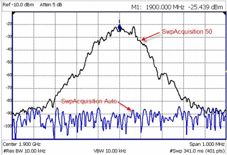
In the graphic above, a GSM signal in a framed data format; timeslot zero ON; all others OFF;
PRF == 218 Hz, Duty Cycle == 12.5%. The pulsed signal becomes visible on every sweep update with SwpAcquisition == 50.
SwpAcquisition is NOT an absolute measure of time, but a relative number between 1 (fastest) and 5000 (slowest) sweep time. The actual time that was required to complete a sweep is annotated on the screen.
1.Press Sweep 3.
2.Then SwpAcquisition Auto Man.
3.Then choose from the following:
—Auto Sweep is set to the fastest sweep possible with the current settings.
—Man Enter a relative acquisition value between 1 and 5000, where:
—Man Enter a relative acquisition value between 1 and 5000, where:
—1 == Fastest sweep possible
—5,000 == Slowest sweep possible
—# is shown in front of the actual sweep time to indicate a manual setting.
Some Detector and Video Bandwidth settings will raise the Auto Sweep Acquisition value greater than 1. In these cases, manually setting Sweep Acquisition lower than the Auto value may have NO effect.
| Measurement speed specifications do NOT apply in Temperature Control mode. Learn more in “Temperature Control Mode” on page 36 |
Learn more about SA mode SwpAcquisition time in the Supplemental Online Help: https://rfmw.em.keysight.com/wireless/helpfiles/FieldFoxOnlineSupplementalHelp/Home.htm.
Two primary settings are responsible for the sweep time: Res BW and SwAcquisition.
—When the sweep time exceeds 1200 seconds (20 minutes), an informational message: Alert: Very long sweep in progress… is annotated on the screen for the duration of the sweep.
—When the sweep time exceeds 4000 seconds (about 1 hour), Meas UNCAL is annotated on the screen. Accuracy cannot be guaranteed.
—InstAlign is always performed only at the beginning of the sweep regardless of the sweep time. Learn more in “How to Access Individual Alignments” on page 223.
When setting the frequency span to Zero, there is NO spectrum of frequencies to display, so the X-axis units becomes Time. The SA becomes like a tunable oscilloscope, with the center frequency being the frequency of interest. This capability is useful for analyzing modulation characteristics, such as pulsed measurements.
For non-zero span measurements, refer to “Sweep Acquisition” on page 202
Figure 9-20 GSM Signal, Framed Data Format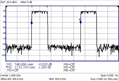
The graphic above shows a GSM signal, framed data format, with timeslot 0 and 3 “on”. Sweep Time is set to approximately the frame interval. Press Single several times until the waveform section of interest is viewable and stable. Then markers can be used to measure the timeslot width and interval as shown.
—Set Center to the frequency of interest
—then set Span to 0 Hz
—or select Zero/Last Span. Each key press toggles the frequency span between 0 Hz and the last specified frequency span.
How to change Sweep Time in Zero Span
—Press Sweep 3
—Then Sweep Time
—Enter a value using the numeric keypad. Sweep time is limited to 1000 seconds for N991xD/3xD models and 6000 seconds for N995xD/6xD models.
—Then select a multiplier key. Learn more in “Multiplier Abbreviations” on page 53.
Learn more about SA mode Sweep Time in the Supplemental Online Help: https://rfmw.em.keysight.com/wireless/helpfiles/FieldFoxOnlineSupplementalHelp/Home.htm.
Triggering SA STEP sweeps do not have trigger behavior. So, they are essentially always in “FREERUN" mode. If you try to set a trigger (other than FREERUN) in SA Step sweep, the FieldFox displays the following popup message:
"Note: Trig Type has no effect while in STEP sweep mode"
External, Video, and RF Burst triggering allows you to initiate an SA mode sweep using an external event such as a signal burst.
All three trigger types can be used in either Zero Span (time domain) or FFT frequency sweeps. Learn more in “Zero Span Measurements” on page 204. Learn more in “Sweep Type” on page 198.
FFT Gating is available for non-zero span measurements. Learn more about FFT Gating in “FFT Gating (Opt 238)” on page 210.
Trigger Type
—Press Sweep 3 > Trigger Settings > Trig Type
—Then choose from the following:
—Free Run Triggering is provided by the FieldFox internal circuitry. A new sweep begins when the previous sweep ends.
—External A sweep is triggered on an external TTL signal at the Ref In/Trig In connector on the FieldFox top panel. Choose to trigger on the rising slope at about 1.7 V or on the falling slope at about 1.0 V using the Trigger Slope setting (below).
—Periodic sets a trigger that repeats at the period rate entered. Periodic trigger's phase can be altered by the Offset value.
The following two selections are similar in that they both trigger a sweep from a signal at the SA RF Input connector. Experiment with both selections to find the best trigger type for your application.
—Video A sweep is initiated when the displayed amplitude of an incoming signal crosses the settable Trigger Level. This selection can detect low-amplitude signals, but also has been filtered considerably and may not be a true representation of the incoming signal.
—RF Burst A sweep is initiated when the signal at the third IF (analog) stage crosses the settable Trigger Level. This selection offers a wider bandwidth and may be a better representation of the incoming signal than Video trigger. However, RF Burst is not as sensitive to triggering on low-level signals.
Sync This softkey is ONLY available when Trigger Type is set to Periodic. SA STEP sweeps do not have trigger behavior. So, they are essentially always in “FREERUN" mode. If you try to set a trigger (other than FREERUN) in SA Step sweep, the FieldFox displays the following popup message:
"Note: Trig Type has no effect while in STEP sweep mode"
Selects the type of signal the periodic trigger is synchronized.
—None No synchronization is selected for a Periodic trigger.
—External A sweep is triggered on an external TTL signal at the Ref In/Trig In connector on the FieldFox top panel. Choose to trigger on the rising slope at about 1.7 V or on the falling slope at about 1.0 V using the Trigger Slope setting (below).
—RF Burst uses an alignment process which is performed in the background to set the detected signal level accuracy. Learn more in “RF Burst Amplitude Alignment” on page 224.
—1 PPS GNSS Periodic trigger is synchronized to a 1 pulse per second GNSS signal.
Trigger Slope This softkey is unavailable when Trigger Type is set to Periodic.
Trigger Slope determines which edge of an External, Video, or RF Burst trigger signal initiates a sweep.
1.Press Sweep 3 > Trigger Settings > Trig Slope
2.Then choose from the following:
—Pos Sweep is triggered by the rising (positive) edge of signal.
—Neg Sweep is triggered by the falling (negative) edge of signal.
Trigger Delay
After a valid trigger signal is received, the sweep begins after the specified Trigger Delay time.
To see the rising edge of a repetitive signal which is triggered on that edge, enter a negative trigger delay value (also known as pre-trigger). Adjust the sweep time to observe the pre-trigger time if necessary.
1.Press Sweep 3 > Trigger Settings > Trig Delay
2.Enter a value using the numeric keypad, the arrows, or the rotary knob.
3.Then select a multiplier key or press Enter. Learn more in “Multiplier Abbreviations” on page 53.
In Zero span, you can use Trigger Position as an easy way to set Trigger Delay by positioning the trigger event on the FieldFox screen. See “Triggering” on page 206.
Period This softkey is ONLY available when Trigger Type is set to Periodic.
Sets the length of time in seconds before a waveform repeats. (Default == 20.00 ms).
Offset This softkey is ONLY available when Trigger Type is set to Periodic.
Sets the periodic trigger offset. (Default == 0.00s)
Trigger Level
Used with Video and RF Burst triggering, a sweep is initiated when an incoming signal crosses this level. The units depend on the Units setting. Learn more in “Scale and Units” on page 165.
RF Burst Trigger Level uses an alignment process which is performed in the background to set the detected signal level accuracy. Learn more in “RF Burst Amplitude Alignment” on page 224. Video Trigger Level is a zero span signal level comparison. Therefore, the sweep will trigger close to the displayed level in zero span measurements. In non-zero span measurements, processing can cause broadband signal energy to display at lower power levels than the originating time domain signal. Therefore, you may need to set the trigger level higher than the displayed level.
1.Press Sweep 3 > Trigger Settings > Trig Level
2.Enter a value using the numeric keypad, the arrows, or the rotary knob.
3.Then select a multiplier key or press Enter. Learn more in “Multiplier Abbreviations” on page 53.
While waiting for a valid trigger signal, Wait is annotated in the top left corner of the FieldFox screen.
If a valid trigger signal is not received before the specified Auto Trig Time, a sweep will occur automatically.
Enter 0 to set Auto Trigger OFF. When Auto Trigger is OFF, the FieldFox does NOT sweep unless a valid trigger signal is received.
1.Press Sweep 3 > Trigger Settings > Auto Trigger [current setting]
2.Enter an Auto Trig Time using the numeric keypad.
3.Then select a multiplier key. See “Multiplier Abbreviations” on page 53.
Trigger Position
Available ONLY in zero span measurements, this setting is an easy way to automatically set the Trigger Delay by positioning the trigger event (also known as T-zero) at any graticule along the X-axis. With T-zero in the center of the screen, you can zoom in and out by increasing or decreasing the sweep time. Using the Trigger Position and Sweep Time settings is a quick and efficient way to examine artifacts of a pulse, much easier than trying to set the Trigger Delay manually.
When Trigger Position is set to OFF, the Trigger Delay softkey is not available. The amount of Trigger Delay that is being used is displayed on the softkey. The Trigger Position is annotated on the screen. Learn how in the following section.
1.Press Sweep 3 > Trigger Settings
2.Then Trig Position. If Sweep Time is longer than 0.15 sec, this softkey is grayed out.
—ON: The position of T-zero is set by the trigger delay.
—OFF: Select, then enter a position value from 0 to 10 using the numeric keypad, the arrows, or the rotary knob.
—0: T-zero occurs at the left graticule.
—5: T-zero occurs at the center of the screen.
—10: T-zero occurs at the far right graticule.
—Then press Enter.
Trigger Settings Annotation
Trigger settings are annotated on the FieldFox screen as highlighted in red in the following image: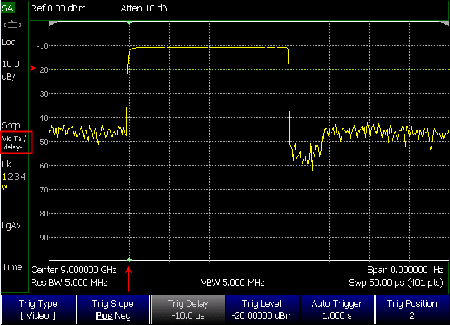
—Square: Trig Type (VidT), AutoTrigger (a), Pos Slope (/), Neg Delay (delay-)
—Horizontal arrow: Trig Level (green horizontal graticule at -20 dBm)
—Vertical arrow: Trig Position T-zero indicators (green arrows at 2nd vertical graticule)
FFT Gating (Opt 238)
Time-gated spectrum analysis allows you to obtain spectral information about signals occupying the same part of the frequency spectrum that are separated in the time domain. Using an external trigger signal to coordinate the separation of these signals, you can perform the following operations:
—Measure any one of several signals separated in time; for example, you can separate the spectra of two radios time-sharing a single frequency.
—Measure the spectrum of a signal in one time slot of a TDMA system.
—Exclude the spectrum of interfering signals, such as periodic pulse edge transients that exist for only a limited time.
FFT Gating is a simple, efficient way to set the proper amount of trigger delay and capture time so that signal artifacts of a repeating waveform or pulse can be examined in the frequency domain. Learn more about trigger settings in “Triggering” on page 206.
For best results, Auto Trigger should be used with this feature to ensure that the sweep does not wait indefinitely for a trigger. Set Auto Trigger to a time that is longer than the expected periodic rate of the signal. This is especially important when using RF Burst or Video triggering in wider spans, because the signal providing those triggers has limited bandwidth. Learn more about Auto trigger in “Auto Trigger Time” on page 209.
For more conceptual information on this topic, please refer to Spectrum Analysis Basics (App Note 150), pages 31 - 35, at https://www.keysight.com/us/en/assets/7018-06714/application-notes/5952-0292.pdf.
How to set FFT Gating
1.Create a non-zero span measurement. Wider frequency spans take more time to acquire.
2.Press Sweep 3 > Trigger Settings > FFT Gating Setup
3.Then choose from the following:
—Gate View OFF ON When ON, a separate zero span measurement is displayed below the non-zero span window. The gate view measurement helps to configure the gate width and delay by revealing (with green markers) the location of the gate relative to the trigger event. The zero span measurement is tuned to the center frequency of the non-zero span measurement with about 5 MHz of bandwidth. The Y-axis scale is the same for both windows.
—Gate View Time Set the X-axis span for the non-zero span window. Enter a value using the numeric keypad, the arrows, or the rotary knob. This value is annotated as Swp (nn) below the window.
—FFT Gating OFF ON When ON, the trigger type, gate width, and delay are applied to the non-zero span measurement. The Res BW is set to a value that is inversely proportional to the gate width.
—Gate Width Set the width of the gating area within the non-zero span window. The gating area is indicated by two vertical green lines. Enter a value using the numeric keypad, the arrows, or the rotary knob.
—Gate Delay Effectively moves the gating area left (negative delay) or right (positive delay) relative to the trigger event. Enter a value using the numeric keypad, the arrows, or the rotary knob.
When you have properly setup the Gate Trigger, Width, and Delay using the Gate View measurement, you can turn Gate View OFF to return to the full screen non-zero span measurement with FFT Gating ON, the RBW set, and the Trigger settings active.
This setting determines whether the FieldFox measures continuously or only once each time the Single or Run / Hold +/- button is pressed. Use Hold / Single or to conserve battery power or to allow you to save or analyze a specific trace.
How to set Single or Continuous
1.Press Sweep 3.
2.Then choose one of the following:
—Continuous
—ON Causes the SA to make continuous sweeps. This is the typical setting for making measurements. Each Run / Hold +/- press causes the SA to toggle between continuous sweep and Hold.
—OFF Causes the SA to Hold. Each Run / Hold +/- or Single press causes the SA to make ONE sweep, then Hold. The Hold annotation changes to an arrow --> while the sweep occurs.
—Single Automatically sets Continuous OFF and causes the SA to make ONE sweep, then Hold.
—Restart Resets the Average counter to 1. The Average counter also is used with MaxHold and MinHold Trace States. Learn more in “Average Count” on page 218.
Points is the number of measurements that are displayed along the X-axis. The higher number of data points, the better the ability to resolve closely spaced signals and the slower the sweep speed.
1.Press Sweep 3 > Points [current setting]
2.Then choose from:
—101 | 201 | 401 | 601 | 801 | 1001
—# Points to enter a trace points value manually (Maximum == 20001).
Trace Display States (SA mode)
In SA mode you can display up to four of the following types of trace states. All SA trace settings can be independently reset (either automatically, or manually) for each trace counter (MaxHold, MinHold, or Average) without resetting any other traces.
Additionally, this independent trace feature provides:
—annotates ONE such trace counter as the minimum trace count of all of the traces (even if multiple counters are active)
—automatically RESET any single Trace counter when parameter couplings dictate that a counter needs to be reset (e.g., TraceMode or TraceDetector changes)
—enables a user to manually reset a single Trace, via the Trace State menu selection (6 Trace > State)
—a manual reset is performed by pressing the same trace State again (i.e., trace state is already enabled), and the selection softkey says “Reset” or “Reset Count” as a hint to the user
Figure 9-21 Trace State Reset Softkeys
A color-coded legend for displayed traces is visible in the left pane of the SA mode screen:
W == Clear/Write; M == MaxHold; m == MinHold; A == Average; V == View
How to display the Trace States
1.Press Trace 6.
2.Then Trace 1,2,3,4 repeatedly to select a trace number to display or change its state. Traces are displayed in the following colors:
—Trace 1 – Yellow Trace 2 – Blue
—Trace 3 – Orange Trace 4 – Green
3.Then State [current setting]
4.Then choose from the following Trace States:
—Clr /Wr (Clear/Write) Displays the actual measured data for each sweep.
—MaxHold Displays the maximum response of the input signal at each data point over multiple sweeps. See also Average Count in “Average Count” on page 218.
—MinHold Displays the minimum response of the input signal at each data point over multiple sweeps. See also Average Count in “Average Count” on page 218.
—Average Each data point is averaged over multiple sweeps as set by the Average Count setting. Learn more in “Average Count” on page 218.
—View Displays and then holds the last complete measurement trace on the screen. This is similar to storing a trace in memory.
—Blank Displays no trace.
5.Press Default All to return all traces to their default settings: Trace 1 (Clear/Write); all other traces (Blank).
| Trace 4 data WILL be overwritten by the FieldFox when using the Independent Source Normalize feature (“Independent Source/Tracking Generator ” on page 192) or using Field Strength antenna or cable corrections (“Field Strength Measurements” on page 169) |
Detection Method SA mode is capable of multiple simultaneous detector setup. Multiple trace detectors are NOT available when: – the FieldFox is set to Zero Span – Channel Measurements are enabled (i.e., Channel Power, Occupied Power, Adjacent Channel Power, and Spectrum Emission Mask) – Whenever Trace Playback is enabled (i.e., Chanel Measurements and Trace Playback are single trace only.) Learn more, see Figure 9-23 on page 216.
In SA modes, the X-axis is comprised of data points, also known as “buckets”. Learn more in “Points ” on page 212.
Regardless of how many data points are across the X-axis, each data point must represent what has occurred over some frequency range an d time interval.
From the frequency span of the measurement, the span of each data point is calculated as (frequency span / (data points-1)). The detection method allows you to choose how the measurements in each bucket are displayed.
Figure 9-22 Detection using One Bucket 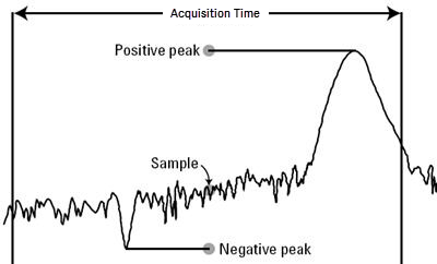
In the graphic above there is one bucket showing Positive peak, Sample, and Negative peak Detection methods.
Figure 9-23 Single and Multiple Detection Annotation - Examples
The current Detection method for each trace is labeled on the left edge of the screen. When a method is selected manually, a # is displayed above the trace’s label. For example: #Nrm means that Normal was selected from the softkeys.
1.Press Trace_6 > Trace Detector
2.Then choose from the following:
—Auto [...] Displays the most appropriate Detection method based on other settings. [# is NOT shown]
—Normal [#Nrm] Provides a better visual display of random noise than Positive peak and avoids the missed-signal problem of the Sample Mode. Should the signal both rise and fall within the bucket interval, then the algorithm classifies the signal as noise. An odd-numbered data point displays the maximum value encountered during its bucket. An even-numbered data point displays the minimum value encountered during its bucket. If the signal is NOT classified as noise (does NOT rise and fall) then Normal behaves equivalently as Positive Peak.
—Positive Peak [#Pk] Displays the maximum value of all the measurements in each bucket. This setting ensures that no signal is missed. However, it is not a good representation of the random noise in each bucket.
—Negative Peak [#NPk] Displays the minimum value of all the measurements in each bucket.
—Sample [#Smp] Displays the center measurement of all the measurements in each bucket. This setting gives a good representation of the random noise in each bucket. However, it does not ensure that all signals are represented.
—Average [#Rms] Displays the Root Mean Squared (RMS) average power of all the measurements in each bucket. This is the preferred method when making power measurements.
Repeat the detection setup process as needed for up to 4 traces and 4 detection methods.
Average Type
In SA mode, there are four different processes in which Averaging is performed:
—Average Traces – Learn more in “Averaging” on page 233.
—Detection Method Averaging – Learn more in “Detection Method” on page 215.
—Noise Marker Averaging - Learn more in “Noise Marker” on page 227.
—Video BW filtering (for non-Zero Span measurements) - Learn more in “Video Bandwidth (Video BW)” on page 197.
There are three types of mathematical averaging that can be performed – Log, Linear, or Voltage (see “How to set Average Type” on page 217). Select ONE of these types and it is used for all of the above averaging processes.
1.Press Meas Setup 4 > Average Type [current setting]
2.Then choose from the following:
—Auto - The FieldFox chooses the most appropriate type of averaging for the current settings. When Detection Method is set to Average, a Noise Marker is present, or a Channel measurement is active, then Power Average is ALWAYS selected. Otherwise, Log Average is selected.
—Log Averaging – Best for displaying Trace Averaging. #LgAv is shown on the left side of the FieldFox screen when selected.
—Power (Linear) Averaging – Best for measuring true power levels. Used in Detection Average and Noise Marker Average. Mathematically, trace noise is 2.5 dB higher than when using Log Average. PAvg is shown on the left side of the FieldFox screen when selected.
—Voltage Averaging – Converts the amplitudes to a magnitude unit before averaging (e.g., Volts, Amps, microVolts, milliVolts, etc.) #VAvg annotation is displayed.
The Average Count setting is used mainly with the Average Trace State described in “Trace Display States (SA mode)” on page 213. In this Trace State, the Average Count setting determines the number of sweeps to average. The higher the average count, the greater the amount of noise reduction.
When Trace (display) State is set to Average, MaxHold, or MinHold, the average counter is shown in the left edge of the screen below the Average Type.
For all three of these Trace States, when Sweep 3 Continuous is set to OFF, press Restart to reset the sweep count to 1, perform <n> sweeps, then return to Hold.
1.Press Meas Setup 4 > Average Count
2.Enter a value from 1 to 10,000 using the numeric keypad, the arrows, or the rotary knob.
3.Press Enter
Alignments To better reflect the enhancements implemented during the alignment process, for firmware versions >A.10.15 “IF Flatness Alignment” is now referred to as “Channel Equalization” or “Channel Equalization Alignment” (ChanEQ Alignment).
This section contains the following:
—“All Alignment and Align All Now” on page 222
—“Individual Alignments” on page 222
The alignments softkeys are located by pressing the Cal 5 hardkey.
All Alignment or Align All Now corrects for receiver drift over temperature and time. SA measurement applications monitor changes in internal temperature and the time since last alignment update and trigger the need for a new update when the alignment becomes stale. The alignment is deemed stale after a significant change in temperature or a significant time elapsed from the last update. The temperature change and time duration necessary to trigger an alignment update is predetermined in the factory. Until the update is performed, annotation indicating “questionable amplitude” is displayed AMPTD?.
When All Alignment is enabled (by default) the FieldFox performs an alignment process using the internal RF source. Although some sweeps are delayed, measurement results are never disturbed.
If the Independent Source (tracking generator) is enabled for your measurement, it will be borrowed to perform the alignment. Again, the measurement results are not disturbed. Learn about the Independent Source in “Independent Source/Tracking Generator ” on page 192.
The alignment process can be disabled. You may want to do this, for example, if you are analyzing the amplitude stability of a signal.
SA and all modes built on its infrastructure require three types of alignments:
—InstAlign Amplitude Alignment
—RF Burst Amplitude Alignment
—Channel Equalization
These are referred to as Individual Align.
All three or a subset of the individual alignments are required for each specific mode, depending on the type of measurement supported by it:
SA:
—InstAlign Amplitude Alignment
—RF Burst Amplitude Alignment
RTSA:
—InstAlign Amplitude Alignment
—WidePath Burst Trigger Alignment
—Channel Equalization
Channel Scanner:
—InstAlign Amplitude Alignment
EMI Measurements:
—InstAlign Amplitude Alignment
—WidePath Burst Trigger Alignment
—Channel Equalization
ERTA:
—InstAlign Amplitude Alignment
IQA:
—InstAlign Amplitude Alignment
—RF Burst Amplitude Alignment
—Channel Equalization
Built-in Power meter
—InstAlign Amplitude Alignment
Default settings and recommended use model for many applications:
—Coupled individual alignments
—Coupled state is Auto
—Individual alignments are not accessible via front panel soft-keys
—Individual alignments cannot be UnCoupled
For special cases, the individual alignments can be accessible via the front panel soft-keys using the Preference setting SA - Individual Alignment Control > On/Off. This enables a soft-key for access to Individual Alignments when this preference is set to ON: Cal 5 > Individual Align. For more refer to “Preferences” on page 870, in Chapter 31 System Settings.
The individual alignments may be:
—Coupled (default) - when they are in the same state, or
—Uncoupled - when at least one of them is in a different state than the other ones
—Executed on demand, all of them, using the Align All Now softkey.
Each of the individual alignments:
—could be in one of three states:
—Off - the alignment is not applied and is not updated automatically
—Auto (default) - the alignment will be updated over time and temperature as needed, no user interaction required
—Hold - the unit holds the alignment values from the last alignment-execution and does not execute another alignment automatically
—can be updated on demand using the corresponding Align Now soft-key. Refer to “Individual Alignments” on page 222.
—The All Alignment soft-key has the following functionality:
—when the individual alignments are Coupled, the state of all of them can be changed simultaneously using the All Alignment soft-key sub-menus
—when the individual alignments are UnCoupled, they will be coupled when using the All Alignment soft-key sub-menus and their state will be simultaneously changed accordingly
All Alignment and Align All Now
| IMPORTANT! It is recommended that you use Align All Now, because it includes the individual alignment InstAlign Amptd Align Now, as well as, Burst Align Now, and ChanEQ Align Now. But, if you would prefer to have manual control over the individual alignments, then refer to the SA Individual Alignment Control setting in “Preferences” on page 870, in Chapter 31 System Settings. The notification AMPTD? displayed on screen means the InstAlign amplitude alignment or channel equalization is stale (if its state is Hold) and requires an update or it is in the OFF state. This situation does not occur when the respective alignment is in the Auto state. To clear this notification, press the Align All Now softkey. |
How to set All Alignment and Align All Now
—Press Cal 5
—Then All Alignment [Auto] (to enable or disable the All Alignment) – Default is Auto.
—or
—Then Align All Now (to manually perform an Align All Now.) This performs an alignment on all three individual alignments: Amptd Align Now, Burst Align Now, and ChanEq Now). Refer to “Individual Alignments” on page 222.
—Press Back
If you want to disable the All Alignment [Auto], you can do so in the FieldFox preferences (i.e., you may want to do this, for example, if you are analyzing the amplitude stability of a signal).
Refer to the SA Individual Alignment Control setting in “Preferences” on page 870, in Chapter 31 System Settings. See also, “Individual Alignments”.
| IMPORTANT! It is recommended that you use All Alignment [Auto] or Align All Now in lieu of the individual alignments (Amptd Align Now, Burst Align Now, and ChanEQ Align Now), because All Alignment [Auto] and Align All Now includes the individual alignment InstAlign Amptd Align Now, Burst Align Now, and ChanEQ Align Now. But, if you would prefer to have manual control over the individual alignments, then refer to the SA Individual Alignment Control setting in “Preferences” on page 870, in Chapter 31 System Settings. The Individual Alignment softkey is only available, when the preference SA - Individual Alignment Control is set to On in the FieldFox Preferences menu. Refer to “Preferences” on page 870, in Chapter 31 System Settings. |
How to Access Individual Alignments
This section assumes access to individual alignments was activated using the FieldFox’s system settings’ Preferences. Once enabled, an Individual Alignments softkey is displayed. Refer to “Preferences” on page 870, in Chapter 31 System Settings.
1.Press Cal 5
2.Then Individual Align
3.Then Amptd Align Now or
Then Burst Align Now or
Then ChanEq Align Now
4.Press Enter
How to make Amplitude Alignment settings
| During continuous sweep (“acquisition” for IQA) operation, automatic Alignments will NOT interrupt the ongoing measurement, but when necessary, will occur opportunistically as settings are changed. When no automatic alignment updates occur, existing alignments can become stale over time and temperature drift, so a warning annotation on the left panel will light up indicating that alignments need updating. |
SA, IQA, RTSA, and other modes use a proprietary amplitude alignment algorithm to make extremely accurate amplitude measurements over the full frequency range of the FieldFox.
These settings do NOT survive a Preset or Mode Preset.
1.Press Cal 5 > Individual Align > Amptd Alignment
2.Then choose from the following:
—Auto (Default setting) Alignments are required and are performed automatically, when necessary, at times when interrupting the RF Output is deemed acceptable. The alignment process is performed opportunistically when changes in settings require the measurement to stop momentarily and a significant time elapsed since the last alignment (predetermined in the factory) or the internal instrument temperature has changed sensibly (predetermined in the factory).
Some examples of the conditions when alignments occur are: This could be a Center frequency change, or it could be as simple as requesting a Single sweep. Also, unique alignments are required at different FieldFox receiver frequency bands, so even if the temperature hasn't changed, an alignment may be required when one changes the Center frequency.
If a needed alignment cannot be performed, the user is notified about questionable amplitude AMPTD?.
—OFF Alignments are not performed. The most recent alignment result is cleared. Only factory corrections are applied to SA Receiver measurements. Questionable amplitude AMPTD? is always displayed.
— Hold The alignment process is stopped, but the last alignment values are applied to subsequent sweeps.
—Amptd Align Now An alignment is performed immediately, thus updating (clearing) any questionable amplitude status. If the Mode was previously Off, it is changed to Hold.
Amptd? is annotated in the lower left corner of the FieldFox screen when amplitude alignment is questionable. This is always true when OFF, and is conditionally true in Auto or Hold when the most recent alignment is deemed stale.
RF Burst Amplitude Alignment
RF Burst alignment calibrates the circuitry to provide accurate external RF Burst triggering. Learn more about RF Burst triggering in “Triggering” on page 206.
When enabled (by default) the FieldFox performs an alignment process using the internal RF source. Although some sweeps are delayed, measurement results are never disturbed.
If the Independent Source is enabled for your measurement, it will be borrowed to perform the alignment. Again, the measurement results are not disturbed. Learn about the Independent Source in “Independent Source/Tracking Generator ” on page 192.
The alignment process can be disabled. You may want to do this, for example, if you are analyzing the amplitude stability of a signal.
How to use Burst Alignment settings
These settings do NOT survive a Preset or Mode Preset.
1.Press Cal 5 > Individual Align > Burst Alignment
2.Then choose from the following:
—Auto (Default setting) SA measurement applications monitor changes in internal temperature and the time since last alignment update and trigger the need for a new update when the alignment becomes stale. The alignment is deemed stale after a significant change in temperature or a significant time elapsed from the last update. The temperature change and time duration necessary to trigger an alignment update is predetermined in the factory.
—OFF The alignment process is NOT performed. Only factory correction values are used.
—Hold The alignment process is stopped, but the last alignment values are applied to subsequent sweeps.
Burst Align Now An alignment is performed once and applied to subsequent sweeps.
Channel Equalization (IQA and RTSA Only) During continuous sweep operation for RTSA and continuous acquisition for IQA, automatic Alignments will NOT interrupt the ongoing measurement, but when necessary, will occur opportunistically as settings are changed. When no automatic alignment updates occur, existing alignments can become stale over time and temperature drift, so a warning annotation on the left panel will light up indicating that alignments need updating. When alignments need updating, you will see a “Channel Equalization” or “ChanEq” error message displayed.
IQA and RTSA modes use proprietary channel equalization algorithms to make extremely accurate channel measurements over the full frequency range of the FieldFox.
How to use Channel Equalization Alignments settings
These settings do NOT survive a Preset or Mode Preset.
1.Press Cal 5 > Individual Align > ChanEq Alignment
2.Then choose from the following:
—Auto (Default setting) SA measurement applications monitor changes in internal temperature and the time since last alignment update and trigger the need for a new update when the alignment becomes stale. The alignment is deemed stale after a significant change in temperature or a significant time elapsed from the last update. The temperature change and time duration necessary to trigger an alignment update is predetermined in the factory.
Some examples of the conditions when alignments occur are: This could be a Center frequency change, or it could be as simple as requesting a Single sweep. Also, unique alignments are required at different FieldFox receiver frequency bands, so even if the temperature hasn't changed, an alignment may be required when one changes the Center frequency.
—Hold The alignment process is stopped, but the last alignment values are applied to subsequent sweeps.
—OFF The alignment process is NOT performed, and the channel equalization is deactivated.
When you press ChanEq Align Now An alignment is performed immediately.
The Amptd? annotation lights up whenever the current channel equalization is deemed stale.
A display line is a simple, horizontal line that can be placed at any amplitude level on the SA screen or set to any level in IQA. Use a display line as mental guide for visual feedback. A display line is similar to a Limit Line, except that no PASS/FAIL testing occurs. A display line is easier to create than a Limit Line. Learn more in “All about Limit Lines” on page 834.
Figure 9-24 Display Line with Annotations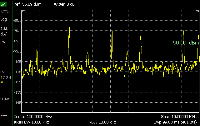
How to create and move a Display Line
1.Press Limit 8 > Display Line OFF ON
2.Then enter a Y-axis value using the arrows or the rotary knob, then press Enter. Or enter a value using the numeric keypad and press a suffix key or press Enter.
Learn more, “All about Limit Lines” on page 834.
For comparison purposes, electronic noise measurements are often displayed as though the measurement was made in a 1 Hz Res BW. However, making an actual measurement at a 1 Hz Res BW is extremely slow.
A Noise Marker, unique to SA mode, mathematically calculates the noise measurement as though it were made using a 1 Hz bandwidth.
Several data points (or ‘buckets’) are averaged together to calculate the Noise Marker readout. To accurately measure noise, the Noise Marker should NOT be placed on, or too close to, a signal. The distance from a signal depends on several factors. To know if an accurate reading is being made, move the Noise Marker until consistent measurements are displayed in adjacent data points.
In addition, when a Noise Marker is displayed, the Detection method is automatically switched to Average and PAvg is shown on the FieldFox screen. This occurs only when Detector is set to Auto. Learn more in “Detection Method” on page 215.
With a Noise Marker present, the Res BW can be changed and the displayed noise floor will also change, but the Noise Marker readout will remain about the same.
Noise Markers can be used like regular markers. A Noise Marker is distinguished from a regular marker by (1Hz) after the marker readout value. Learn more about regular markers in “All about Markers” on page 819.
How to measure Noise with a marker
1.Press Marker to create or select a Normal or Delta marker to use to measure Noise.
2.Then More > Marker Function > Noise ON OFF.
Power Spectral Density (PSD) Function (SA mode Only)
The Power Spectral Density Function (PSD Function) is a way to normalize the SA measurement to a 1 Hz Bandwidth. Every SA Resolution Bandwidth is characterized by an “Equivalent Noise Bandwidth” (ENBW) that in general is a few percent wider than the Resolution Bandwidth itself. To normalize the measurement to this ENBW, an offset is added in this amount:
PsdOffset = -10 * Log10( ENBW )
This offset is added to the Reference Level, the Trace values, and Marker values and suffix annotation is updated with “/Hz” or “(1Hz)” as an indication that the results are now normalized to 1Hz. This is similar to what the Noise Marker function does, but the Noise Marker also first averages several trace points around the marker location. Similar to a Noise Marker, the PSD Function will also auto-couple the Detector to RMS.
See also, “Noise Marker” on page 227.
Learn more, see “Creating and Importing *.csv Limit Line Files” on page 841.
How to measure the PSD function:
—Press Scale/Type > More > PSD Function ON OFF (Default == OFF).
Logarithmic X-axis Interpolation (EMI and SA modes Only)
Normally, limit lines are interpolated linearly between the defined limit points (i.e., as a delta dB per Hz). Sometimes the user may want to change the limit line interpolation so that it is logarithmic vs. X (i.e., as a delta dB per log10(Hz)). The “AUTO” state for this control will automatically switch to logarithmic interpolation, if the Trace is being drawn on a logarithmic frequency axis (Log Freq Axis X, available by Freq/Dist > More for SA and EMI modes). The “OFF” state keeps limit line interpolation happening linearly, regardless of the current choice of logarithmic frequency axisX.
Learn more, see “How to change from Linear to Log Axis View” on page 161.
How to set Logarithmic X-axis Interpolation (Log Freq AxisX)
1.Press Limit 8 > Options > LogX Interp Auto Off – Enables/disables logarithmic interpolation of the X–axis (Default == Auto).
2.Then choose from the following:
—Auto – (default) reacts to the trace data. If the you chooses LogX axis for your trace data, then Auto will cause the interpolation of the Limit Lines to also act “logarithmically vs. X”. But, for normal Linear X axis trace data, the interpolation of the limit line remains as before, straight line interpolation vs. the x axis data.
—Off – forces the limit lines to interpolate linearly vs. X.
A Band/Interval Power marker—available in IQA and SA modes—accumulates the power that is measured over several adjacent data points (or ‘buckets’). The range of buckets being measured is displayed with vertical posts around the marker. This Band Span value is selectable.
This feature is very similar to a channel power measurement (“Channel Power (CHP)” on page 234).
When the frequency span is set to Zero span, the marker is referred to as an Interval Band Marker because it averages power over a specific time interval. In this case the range is specified as the Interval Span. Learn more about Zero span measurements in “Zero Span Measurements” on page 204.
If the Detection method and Averaging type are set to Auto when you enable a Band/Interval Power marker, the Detection method will change to Average (RMS) and Averaging type will change to Power average. Other Detection methods or Averaging type settings will usually cause measurement inaccuracy. Learn more about Detection method in “Detection Method” on page 215, and Averaging Type in “Average Type” on page 217.
Summary:
—In Zero span, an Interval Power Marker yields the average power over the specified time interval.
—In non-Zero span, a Band Power Marker yields the total power over the specified frequency range.
How to measure Band/Interval Power with a marker
1.Press Marker to create or select a Normal or Delta marker to use to measure Band/Interval Power.
2.Then press More > Marker Function > Band/Int Power > Band (or Interval) Span
3.Then choose from the following:
—Auto Measures power over 5% of the displayed span, or ½ graticules. The Band Span is automatically updated to remain at 5% when you change the frequency span.
—Man Enter a frequency or time value using the arrows or the rotary knob, then press Enter. Or enter a value using the numeric keypad and select a frequency or time suffix. The Band Span remains at the frequency or time value that you set as the span changes.
Available in SA mode ONLY. Use any existing marker to make highly-accurate frequency counter readings. For highest accuracy, lock the FieldFox to a stable external frequency reference. Learn how in “Frequency Reference Source” on page 890.
When Frequency Counter is ON, the FieldFox uses background sweeps to zoom on the signal, measure the signal peak with 1 Hz resolution, and display the frequency of the signal peak in the marker annotation area. The marker does not move to the signal peak.
When Freq Counter is ON, measurement sweeps are considerably slower.
How to use Frequency Counter
1.Press Marker.
2.Press Normal, Delta, or Peak, or select an existing marker to use as a frequency counter.
3.Locate the marker somewhere on a CW signal. It does NOT have to be on the peak.
4.Then More > Freq Count ON
5.With Freq Count ON, you can scroll through the existing markers that are located on a discrete CW signal, and read the frequency of the signal peak. However, each frequency count update requires another sweep. If the FieldFox is in HOLD, press Single to update the frequency count results.
This feature was created to allow recall of vintage instrument states (older than Rev. 7.0) that included Zero span sweep with a trigger delay and at least one marker. Before Rev. 7.0, these instrument states were saved and recalled with the equivalent of the ON state of this setting. The default setting is OFF. Learn more about Triggering with negative delay in “Triggering” on page 206.
1.Press Mkr->/Tools > More > Mkr Properties > Time Zero Fixed
2.Then choose from the following:
—ON Time Zero is fixed at the left-edge of the screen. A marker in negative delay resides at this point. This is the vintage behavior.
—OFF (default) Time Zero is located at the T-zero indicators. A marker in negative delay appears to the left of T-zero.
When enabled, the Audio Beep feature emits a repetitive beep sound which varies in tone pitch and repetition rate to indicate the relative power level of the active marker. The highest tone pitch and fastest beep rate occurs when the marker Y-axis position is at the top of the display. Conversely, the lowest pitch and repetition rate occurs at the bottom of the display. Therefore, it is important to scale the signals that you intend to measure between the top and bottom of the screen. Learn more about Scale in “Scale and Units” on page 165.
Audio Beep can be used with any marker type or function, including Band/Interval Power. Learn more in “Audio” on page 876.
How to use Audio Beep
1.Press Marker
2.Optionally, press Marker 1 2 3 4 5 6 to select an existing marker to use with Audio Beep. A marker will be created if one does not already exist.
3.Then More > Marker Function > Audio Beep ON OFF
Audio Beep does NOT beep when the FieldFox is in Hold mode.
While Audio Beep is ON, press Marker 1 2 3 4 5 6 to toggle Audio Beep through the existing markers.
To set FieldFox speaker volume control, press System, then Volume. Learn more in “Audio” on page 876.
Meas UNCAL appears in the lower-left corner of the screen when the FieldFox can NOT display accurate measurement results with the current settings. Usually, the part of the trace that is inaccurate is shown at –200 dB.
The following situation can produce Meas UNCAL:
—When the ResBW/VBW ratio exceeds 10,000, causing the VBW filter to reach the maximum capacity for averaging.
In SA mode, when the current trace does not exactly match the annotation that is on the screen, an asterisk is displayed in the upper-right corner of the screen graticule area. This would occur, for example, when the Res BW setting is changed while in sweep Hold mode. The annotation is changed immediately, but the trace is not updated until the next sweep occurs. Therefore, the current data trace does not match the screen annotation. See the asterisk in Figure 9-1 on page 155.
The following Channel Measurements are offered in SA mode:
Channel Power “Channel Power (CHP)” on page 234
Occupied Bandwidth “Occupied Bandwidth” on page 235
Adjacent Channel Power Ratio “Adjacent Channel Power Ratio (ACPR)” on page 237
Radio Standards and Channel Measurements
To tune the frequency range of any of the Channel Measurements using channels instead of frequency, first select a Radio Standard, then select Units == CHAN. Learn how to select a Radio Standard and channels in “How to select a Radio Standard” on page 161.
When you first select a Radio Standard, then select a Channel Measurement:
—With Units == FREQ selected, the center frequency and span will ALWAYS change to the full frequency range of that standard (Uplink and Downlink) to allow for a quick scan of energy. The X-axis annotation indicates the frequency range.
—With Units == CHAN selected, the FieldFox chooses either the uplink or downlink band, and displays that range of frequencies. You can then tune within that Standard using Start CHAN, Stop CHAN, or Center CHAN. The X-axis annotation indicates the frequency range.
When you first select a Channel Measurement, then select a Radio Standard, the BW, Offset, RRC, Integration BW, and Span settings are changed to those of the standard. In addition, Res BW can also change when set to ‘Auto(couple)’. However, center frequency is NOT changed unless you first select Units == CHAN.
Measurement Preset allows you to easily reset any of the channel measurements to its default settings. The Center Frequency, Preamp ON|OFF, RF Attenuation, Markers, Limits, and Radio Standard settings are NOT reset.
How to select Measurement Preset:
—Press Preset > Mode Preset
By default in ALL Channel measurements, averaging is enabled and set to display the average of the last 15 measurements. When enabled, this average setting is automatically making the following ‘averaging’ settings in order to provide the most accurate power measurements:
—Averaging Type is set to Power.
—Trace State is set to Average.
—Detector is set to Average.
—Count is set to 15.
Any of these settings can be changed manually during a Channel measurement. Learn more about these settings starting in “Average Type” on page 217.
To change Averaging:
1.Press Meas Setup 4.
2.Then Average Enable ON OFF OFF effectively sets the Average Count to 1.
3.Then Average Count
4.Enter a value between 1 and 10,000 using the numeric keypad, arrows, or the rotary knob.
5.Press Enter.
Only one measurement trace can be displayed in Channel Measurements.
Channel Power measures total power over the specified Integrated BW. The Integration Bandwidth (IBW) can be adjusted to measure the power over multiple channels.
Figure 9-25 Channel Power Measurement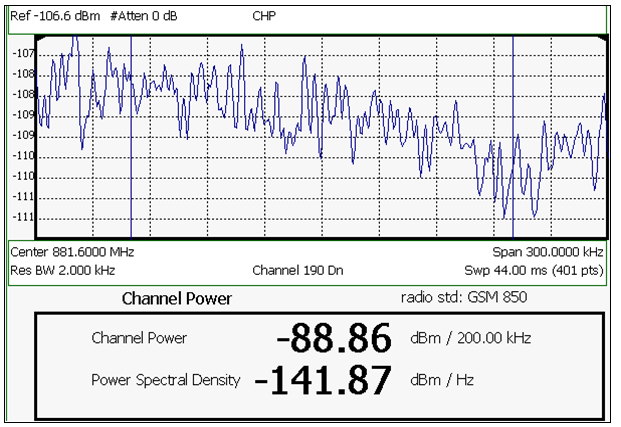
The following two Channel Power levels are displayed:
—Channel Power - measures total power over the specified Integrated BW.
—Power Spectral Density – same measured power, but mathematically normalized to a 1 Hz bandwidth using the same algorithm as Noise Marker. Learn more about the Noise Marker in “Noise Marker” on page 227.
How to select Channel Power
1.Press Measure 1
2.Then Channel Power
When Channel Power is selected, the following settings are maintained from a previous measurement: Center Frequency, Preamp ON|OFF, and RF Attenuation.
Integration Bandwidth
When Channel Power is selected, vertical posts appear on the display to mark the current Integration Bandwidth setting. The displayed Channel Power and Power Spectral Density values are measured and calculated over the specified Integration Bandwidth.
By default, the displayed frequency span is automatically coupled to the Integration Bandwidth. As you change the Integration Bandwidth, the frequency span is adjusted so that the vertical posts appear to NOT move. However, when you manually change the frequency span, the Integration Bandwidth is no longer coupled to the frequency span.
When a Radio Standard is selected, the appropriate Integration Bandwidth is set automatically. Learn more about Radio Standards in “Radio Standard” on page 161.
To change Integration Bandwidth:
1.Press Meas Setup 4 > Integrating BW (Integrating Bandwidth)
2.Enter a value between 100 Hz and 5 GHz using the numeric keypad, arrows, or the rotary knob.
3.Press Enter
Other Channel Power Settings
All relevant FieldFox settings are made automatically to ensure the highest accuracy, such as ResBW, VideoBW, and sweep (SwpAcquisition) speed. These, and all other SA mode settings, can be changed manually in a Channel Power measurement.
—Learn about Measurement Preset in “Measurement Preset” on page 233.
—Learn about Averaging in “Averaging” on page 233.
—Learn about RRC Weighting in “RRC Weighting” on page 241.
Occupied Bandwidth measures the power of the displayed frequency span and displays vertical posts at the frequencies between which the specified percentage of the power is contained. The frequency span between the two vertical posts is the Occupied Bandwidth. The Occupied Power, the power that is contained between the two posts, is also displayed in dBm.
Figure 9-26 Occupied Bandwidth Measurement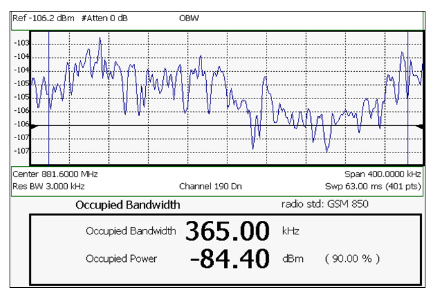
The graphic above shows an OBW measurement; Chan 190 Downlink; GSM850 Radio Standard
How to Select Occupied Bandwidth
1.Press Measure_1
2.Then Channel Measurements
3.Then Occupied BW
When Occupied Bandwidth is selected, the following settings are maintained from a previous measurement: Center Frequency, Preamp ON|OFF, and RF Attenuation.
Frequency Span
Occupied BW is calculated from power that is measured over the entire displayed Frequency Span. The frequency span can be entered using arbitrary frequencies or by using a Radio Standard in conjunction with channel numbers. Learn how to select a Radio Standard and channels in “Channel Selection” on page 162.
To change Frequency Span:
1.Press Freq/Dist > Freq Span
Integration BW (IBW) is coupled to the Frequency Span setting. Frequency Span is 50% wider than the IBW (e.g., if the IBW value is 1 MHz, then the Frequency Span value is 1.5 MHz). |
2.Enter a value using the numeric keypad, arrows, or the rotary knob.
3.Press Enter
Power Percent
This setting specifies the percentage of total measured power to display between the vertical posts. The measurement defaults to 99% of the occupied bandwidth power. The remaining power (1% of default setting) is evenly distributed;.5% of the power on the outside of each side of the vertical posts.
To change Power Percent:
1.Press Meas Setup 4 > Power Percent
2.Enter a value between 10 and 99.99 using the numeric keypad, arrows, or the rotary knob.
3.Press Enter.
Other Occupied Bandwidth Settings
All relevant FieldFox settings are made automatically to ensure the highest accuracy, such as ResBW, VideoBW, and sweep (SwpAcquisition) speed. These, and all other SA mode settings, can be changed manually in a Occupied Bandwidth measurement.
—Learn about Measurement Preset in “Measurement Preset” on page 233.
—Learn about Averaging in “Averaging” on page 233.
Adjacent Channel Power Ratio (ACPR)
ACPR measures the power of a carrier channel and the power in its adjacent (offset) channels. The measurement results can help you determine whether the carrier power is set correctly and whether the transmitter filter is working properly.
You can measure the channel power in one, two, or three adjacent (offset) channels on the low frequency and high frequency side of the carrier channel.
Limits can be used to quickly see if too much power is measured in the adjacent channels.
Figure 9-27 GSM 850-Ch 251-Up with one Offset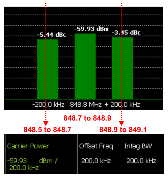
In the graphic above, red frequencies (MHz) are added to illustrate offset and integ BW.
Data in the ACPR graphical chart is always presented in dBm for the carrier, and dBc (dB below the carrier) for the offsets. This can NOT be changed. Use the Meas Type setting (next page) to change how the data is presented in the table below the graph.
How to select ACPR
—Press Measure__1
—Then Channel Measurements
—Then Adjacent Channel Power
When ACPR is selected, the following settings are maintained from a previous measurement: Center Frequency, Preamp ON|OFF, and RF Attenuation.
Frequency Range/Channel
When a Radio Standard is selected, the appropriate center frequency or channel and span is set automatically. The frequency or channel number can then be changed from the Freq/Dist menu. Learn how to select a Radio Standard and channels in “Radio Standard” on page 161.
The frequency range of an ACPR measurement can also be entered using arbitrary frequencies.
When a Radio Standard is NOT selected, the center frequency of a previous measurement is maintained when ACPR is selected.
Changing the Integration Bandwidth
The Integration Bandwidth of the carrier and offsets is the frequency span over which power is measured.
To change Integration Bandwidth:
1.Press Meas Setup 4 > Integrating BW
2.Enter a value between 100 Hz and 100 MHz using the numeric keypad, arrows, or the rotary knob.
3.Press Enter
How to define adjacent (Offset) channels
An offset represents a difference in center frequencies of the carrier channel and its adjacent channel to be measured. The frequency range for each offset is specified with an Offset Freq and Integ BW. Each offset that is created has a Lower (carrier MINUS Offset Freq) and Upper (carrier PLUS Offset Freq) set of frequencies.
1.Press Meas Setup 4 > Offsets
2.Press Offset 1 2 3 to select an offset.
3.Then Offset State to set that offset ON or OFF.
4.Select Offset Freq This is the difference between the carrier center frequency and the center frequency of the offset channel. Then enter a value using the numeric keypad.
5.Select Offset Integ BW This is the frequency range over which power is measured in that offset; half of the range below and half above the Offset Freq.
How to set limits for adjacent channels
You can set a unique threshold power for each of the offsets that will cause a FAIL indication (RED bar). This occurs when the calculated dBc power (on top of the offset bar) is ABOVE the specified level.
To set limits, with an ACPR measurement on the screen:
1.Press Limit 8 > Offset (1,2,3)
2.Then choose from the following:
—LowerOffsetLimit Sets a limit for the lower-frequency offset.
—Upper OffsetLimit Sets a limit for the higher-frequency offset.
3.Then enter a value using the numeric keypad, arrows, or the rotary knob.
4.Then Limit Test ON OFF
Measurement Type
This setting determines how the measured carrier and offset power levels in the table are presented. (Data in the graphical chart is always presented in dBm for the carrier and dBc for the offsets.)
To select Meas Type:
1.Press Meas Setup 4 > More > Meas Type
2.Then choose from the following:
—Total Pwr Ref – Integrated carrier power is represented in dBm, and relative powers between offsets and carrier are represented as dBc (dB below the carrier).
—PSD Ref (Power Spectral Density) – Integrated carrier power is normalized to a 1 Hz density as dBm/Hz using a similar algorithm as Noise Marker. Learn more about the Noise Marker in “Noise Marker” on page 227.
For both Meas Types, choose the reference for the offset data.
3.Press Ref Value to toggle between these settings:
—Auto - dB or dBc value is computed by subtracting the measured carrier power from the measured offset power.
—Man – dB or dBc value is computed by subtracting the entered RefValue from the measured offset power.
—Then enter a value to be used to reference the data using the numeric keypad, arrows, or the rotary knob.
Other ACPR Settings
All relevant FieldFox settings are made automatically to ensure the highest accuracy, such as ResBW, VideoBW, and sweep (SwpAcquisition) speed. These, and all other SA mode settings, can be changed manually in a ACPR measurement.
—Learn about Measurement Preset in “Measurement Preset” on page 233.
—Learn about Averaging in “Averaging” on page 233.
RRC, or Root-Raised-Cosign weighting, is offered with Channel Power and ACPR measurements.
When RRC Weighting is applied to transmitted and received power, the edges of the channel are ‘smoothed’ to help prevent interference. To accurately measure a channel that has RRC weighting, set the same value of RRC weighting as that used in the transmitter and receiver.
Figure 9-28 Channel power measurement with.22 RRC applied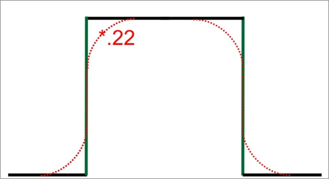
RRC Weighting is set and enabled automatically when included in a selected radio standard.
To set and enable RRC Weighting:
1.Press Meas Setup 4 > RRC Weighting ON OFF > More > RRC Alpha [current setting]
2.Enter a value between 0 (no smoothing) and 1 (most smoothing) using the numeric keypad, arrows, or the rotary knob. A standard level of filtering is 22.
3.Press Enter.
How to Set Up EMF Settings (Requires EMF (Option 358), GPS (Option 307), and SA Mode (Option 233–Mixed Analyzers))
| If OTA or SA mode does not detect an EMF Option 358 license, then the EMF application and the EMF antenna’s axes must be set up manually. This use model is not recommended or supported by Keysight. |
| The EMF antenna’s cable loss is not included, in the antenna’s correction factors. For an accurate EMF measurement, the cable loss values should be accounted for. Refer to “Editing Cable Correction Factors and Adding New Cable Factors” on page 253. |
| IMPORTANT! The EMF antenna, ARIA6000 or FSH3D or equivalent—is required for EMF measurements. Refer to Chapter 15, “USB Antennas – Full Capability Requires EMF Option 358, and either SA mode (Option 233 Mixed Analyzers) or OTA—LTE FDD (Option 370), LTE TDD (Option 371), 5G NR / 5G NR EVM Conducted / 5G TF (Option 378).” |
The antenna operation for single-polarization measurements is different between ARIA6000 and FSH3D. Please consult the datasheet corresponding to each antenna for specific details. |
EMF mode measures signals at the SA RF Input Port 2 connector.
EMF mode requires the FieldFox to have SA mode (Option 233 on combination analyzers), or OTA-LTE FDD (Option 370), LTE TDD (Option 371), 5G NR (Option 378), GPS (Option 307), and CPU2 installed.
Recommended, but not required, preamplifier (Option 235) to improve receiver sensitivity.
With Option 358 (EMF), network designers can measure and verity the RF exposure compliance as required by each country.
If SA mode is licensed for EMF Option 358, the primary measurement performed is Channel Power (CHP) which automatically switches amongst the 3 TriAxial antenna axis (X/Y/Z), to provide a summation of “total power” detected, using unique Antenna supplied corrections for the individual axis, with results in FieldStrength units. This is accomplished within the existing SA Channel Power measurement.
With or without license EMF Option 358, the System Utilities menu enables one to Import Corrections and manually drive the Antenna to a particular axis (X, Y, or Z). The manual control thus allows any SA Receiver measurement to sweep that axis just like any other antenna transducer, however without license the imported corrections are not usable from the Apps. But with license the SA provides for easy use of the imported XYZ corrections, thus allowing presentation of correctly compensated FieldStrength measurements, for 1 axis at a time.
This section reviews the steps in setting up an EMF measurement, using a EMF antenna. If you are not familiar with this process or would like more information, refer to Chapter 15, “USB Antennas – Full Capability Requires EMF Option 358, and either SA mode (Option 233 Mixed Analyzers) or OTA—LTE FDD (Option 370), LTE TDD (Option 371), 5G NR / 5G NR EVM Conducted / 5G TF (Option 378).”
This section consists of:
—“EMF Setup Procedure” on page 245
EMF has the following features:
EMF Measurement Results:
—Measure and display corrected field strength in RMS average power
—Antenna control over X, Y, and Z antenna factors downloaded via USB for ARIA6000 antenna or import a CSV file for FSH3D antenna
—Pass/Fail limit testing supported
—External PC not required
EMF uses the following data formats:
—Field Strength units:
—dBµV/m – For use with E-field signals
—dBµA/m – For use with H-field signals
—dBG – dB Gauss
—dBpT - dB Tesla
Figure 9-29 Example of EMF with Triaxial Antenna
EMF Setup Procedure When the EMF antenna correction factors are imported, EMF (Option 358) couples many settings to ease setting up the EMF measurement (e.g., Apply Corrections is enabled, all X, Y, and Z antenna axes are enabled, and Amp Corr Select is set to ARIA6000 or FSH3D Triaxial XYZ) IMPORTANT! The softkey menu selection and display of Axis X, Y, Z, corresponds to Loop 1, 2, 3, respectively for EMF antenna FSH3D.
1.Setup the FieldFox Spectrum Analyzer for a Channel Power measurement.
a.Press Mode > SA >
b.Press Measure 1 > Channel Measurements > Channel Power
See also, “Channel Measurements” on page 232.
| If necessary, this step can be skipped and done after the EMF antenna is set up |
2.Connect a EMF antenna’s RF cable to the SA RF Input, port 2 and the USB connector to a FieldFox USB port. See also, Figure 9-29 on page 244 and to Chapter 15, “USB Antennas – Full Capability Requires EMF Option 358, and either SA mode (Option 233 Mixed Analyzers) or OTA—LTE FDD (Option 370), LTE TDD (Option 371), 5G NR / 5G NR EVM Conducted / 5G TF (Option 378).”
| Only Agos Advanced Technologies ARIA6000 and Schwarzbeck Mess-Elektronik FSH3D Triaxial Isotropic EMF antenna is currently compatible with EMF (Option 358). |
3.Importing and selecting the X/Y/Z antenna factors:
a.Press System > Utilities > EMF Antennas
—For ARIA6000 EMF antenna, press Antenna Select and select "ARIA6000".
Then press Import Antenna – to import the antenna factors from the antenna’s memory over the USB connection (this may take 5 seconds or so and vary with the triaxial antenna). IMPORTANT! The Import Antenna softkey is only activated when Antenna Select is set to ARIA6000 or FSH3D.
| If the antenna factor import is successful, the FieldFox displays: “Success: Antenna Factors Imported: EMF Antenna ID: ->[R] Antenna ID: ARIA6000-1006 ->[]“. The last 4-digits will vary for each antenna (i.e., “1006” value will vary). If the FieldFox displays this error Error: EMF antenna Error: Not found or Unable to communicate with antenna. Ensure it is connected. is displayed, verify the EMF antenna is connected correctly. See also, “Troubleshooting” on page 495. |
—For FSH3D EMF antenna, press Antenna Select and select "FSH3D".
Then press Import Antenna > Import Files - to import FSH3D antenna factor CSV file from external storage device e.g. USB or SD Card to the INTERNAL storage. Recall File to retrieve these imported CSV files directly from INTERNAL when necessary.
Figure 9-30 FSH3D antenna factor CSV Import Files storage device selection Softkey 
Press the storage device containing FSH3D antenna factor CSV file you wish to import from. The window will navigate to the chosen storage device and display all available CSV files.
Choose a single FSH3D antenna factor CSV file from the list, then press Import.Once imported, press Done to complete the process.
To recall INTERNAL FSH3D antenna factor CSV, press Import Antenna, then select the target CSV file and press Recall File.
| FSH3D antenna factor CSV files MUST be saved in the "AntennaEMF" folder within the storage device to import from. |
—By selecting Antenna Select and choosing either ARIA6000 or FSH3D to verify the EMF antenna selected (Default == Manual). Only compatible EMF antennas can be used for EMF measurements.
See also, “How to Use the Manual EMF Channel Power” on page 250.
—Optional: Press Antenna Axis the antenna axis should be set to Auto for default operation. When AUTO is selected the application (e.g., Channel Power or OTA) controls the axes and switches as needed. With the AUTO setting, all antenna elements (X, Y, and Z) are OFF. The Antenna Axis softkey is only activated when Antenna Select is set to ARIA6000 or FSH3D.
—Press Back > Back to exit the EMF Antenna softkey menu.
4.Enabling the imported EMF antenna factors and Cable factors:
a.Verify that the Channel Power measurement is set: Measure 1 > Channel Measurements > Channel Power
b.To enable the triaxial antenna for EMF: Press Meas Setup 4 > EMF Off > EMF Triaxial [OFF] > Sum All
With Sum All, the field strength from all three axes is summed and displayed. The RF measurements are switched between the three different antennas (three dipoles), and the resulting summation of the total power collected, and averaged.
Alternatively, you can select either of three axes to individually measure the field strength in the one direction.
c.Else, to manually set one of the triaxial antenna’s three axes to individually measure the field strength in one direction.
i.Press Meas Setup 4 > EMF Off > EMF Axis Select [OFF] then
ii.Select a single Axis X, Axis Y, or Axis Z antenna dipole for uncorrected use. [X, Y, or Z] is displayed to indicate which one of the X/Y/Z dipole axes is enabled. If for example the X axis has been selected in the System > Utilities > EMF Antennas menu, then Antenna Axis [X] is displayed to indicate the X axis measurement (i.e., this uncorrected manual mode is typically used when no EMF Option 358 is installed). Refer to Figure 9-31. See also step f.
For corrected manual single axis EMF measurements, refer to “How to Use the Manual EMF Channel Power” on page 250.
Figure 9-31 EMF Axis Select [N] Softkey – With the X–Axis Dipole Selected
d.Modifying the Amplitude Correction Selection:
Press Scale/Amptd > More > Corrections > More then
—Amp Corr Select [TriAxial XYZ] - then choose one of the following:
—Default Receiver side only antenna measurements (Default – when no Tri Axial antenna is detected).
—Src/Rcvr Split to work with non-triaxial receiver and source side antenna measurements.
—Triaxial XYZ (default, when Channel Power is on and when a compatible triaxial antenna’s factors have been imported) for measuring channel measurements and EMF.
—Then <Back to exit to the previous softkey menu.
e.Optional (Tri-Axial XYZ Antenna):
Verifying antenna and cable corrections are applied:
i.Press Scale/Amptd > More > Corrections
—Then verify the Apply Corrections Auto Disabled softkey is set to Auto (This is the default setting when a compatible EMF antenna’s correction factors have been imported, via the System softkeys).
—Then verify the X axis Antenna, Y axis Antenna, and Z axis Antenna are all OFF. These can each be enabled or disabled individually, but for EMF measurements all three axes should be enabled (i.e., Antenna == Off, the applications are setting the X/Y/Z).
—Then Press Cable Off to open the cable correction softkeys menu.
Verify Cable is ON. This can be disabled for applications where an additional cable has not been connected to the triaxial antenna. Before a cable can be used with the EMF measurements it needs to have corrections loaded. If you are going to use a cable, then choose as needed:
—Cable Off to enable a cable for use in your antenna measurement.
—Edit Cable displays a cable corrections table that you can edit
—New displays a cable corrections table that you can edit with new cable correction content.
Yes | – Choose Yes to overwrite the current cable data |
No | – Choose No to exit the cable data edit table view |
—Save Cable Opens a menu to name and save the cable corrections data
—Recall Cable Recalls the selected cable correction file from the \Cables folder.
—Storage Device to select the storage device where your cable correction file is located (Internal/USB/SD Card)
ii.Optional: Press More then
—Press View Corrections OFF ON to turn ON and OFF Pink Trace - Antenna/Cable corrections. This is a composite of all cable/antenna corrections that are currently applied. Available as a useful visual aid, the zero “dB” level (no net correction) is mapped to appear at the -50 dBm on-screen level.
—Press Src/Rcv Split - selecting Src/Rcv Split selects Source and Receiver side measurements.
f.Optional: Example of editing X, Y, and Z axes manually.
| The EMF antenna factors stored in the triaxial antenna itself cannot be overwritten. The antenna factors on FieldFox imported into FieldFox can be modified. To reset the antenna factors in FieldFox to the original factors, re-import the antenna factors |
—Press X axis Antenna – opens the X axis Antenna softkey menus. Then choose one or more of the following:
—X axis Antenna – enable/disable the X axis antenna factors (default is coupled to other settings).
—Edit Antenna – to edit the current imported X factor (if available). Refer to “Editing Antenna Correction Factors and Adding New Antenna Factors” on page 251.
—New – to edit/define a new X factor value. Refer to “Editing Antenna Correction Factors and Adding New Antenna Factors” on page 251.
—Save Antenna – to save either an edited X antenna factor or a new X antenna factor. See also See also Chapter 31, “System Settings” and then to “Alpha Numeric Editing” on page 879.
—Recall Antenna – to recall a stored X antenna factor. See also Chapter 31, “System Settings.”
—Storage Device – to select the location to store your new antenna factor. See also Chapter 31, “System Settings.”
5.Modifying the EMF settings:
Press Meas Setup 4 > More > EMF OFF then
—EMF TriAxial [OFF] disable/enable the EMF tri-axial measurement (Default == OFF)).
—Press Scale/ Amptd > More > Unit dBm choose units (default == dBm).
—Back to exit to the previous softkey menu.
For more details on editing the EMF antenna, refer to Chapter 15, “USB Antennas – Full Capability Requires EMF Option 358, and either SA mode (Option 233 Mixed Analyzers) or OTA—LTE FDD (Option 370), LTE TDD (Option 371), 5G NR / 5G NR EVM Conducted / 5G TF (Option 378).”
How to Use the Manual EMF Channel Power
This manual EMF channel power method procedure is used to adjust the antenna axes when the antennas are to be moved physically and then the X, Y, and Z axes setting values are assigned. The saved results are only accurate as long as User Corrections do not change. The User Corrections include Antenna and Cable compensation, and if those compensations change in any way, it will invalidate the saved measurement results. It is recommended that the Clear Saved Results softkey is pressed for a new equipment setup or the Antenna Corrections are modified. To indicate that a user correction has been changed, an asterisk(*) is displayed to indicate that the Saved results has been compromised and no longer valid.
Importing and selecting the X/Y/Z antenna factors:
1.Press System > Utilities > EMF Antennas
2.Press Antenna Select [Manual] (Default) then
3.Verify you are measuring Channel Power (refer to step 1 on page 245) then
4.Press Meas Setup 4 > EMF Off then
5.Press EMF Axis Select [Off] – to select an antenna axis
6.For this example, press Axis X
The FieldFox display updates to read “X axis Channel Power” and channel power values (dBm /Hz).
7.Move the antenna to the correct physical location/position for your measurement.
8.Antenna corrections: Press Corrections > X-Axis Antenna Off > Antenna OFF to ON – learn more, refer to “How to Use the Antenna and Cable Softkeys” on page 171.
9.When done press <Back
10. Press Meas Setup 4 > EMF Active > Save Axis Result – the display is updated with antenna’s current position channel power values and display trace.
X axis channel power (CHANPOW) data and trace are frozen in the upper right of the EMF Channel Power window.
11. Repeat steps 5 through 10 for the axis Y and Z.
After pressing the Axis Y softkey, the Axis-X Antenna softkey changes to read Enabled (Axis-X measurement saved) and because the Y-Axis is now the active antenna (measuring data). Axis-Y softkey behaves similarly after it is saved and Axis-Z is pressed.
12. Sum Channel Power: Press Save Axis Result. The Live Sum CHP value now displays the summed values of the 3 axes.
Other softkey choices are Restart, Corrections, Clear Saved Results, and Save Traces Blank View.
Editing Antenna Correction Factors and Adding New Antenna Factors
This section contains two procedures illustrating how to edit the Antenna Factors settings table values. If New is selected under the X, Y, or Z Antenna or Cable softkey menu, whatever antenna or cable factors that have been imported as the default values and are displayed in the Settings table
1.Selecting an antenna softkey menu:
Press Scale/Amptd > More > Corrections then choose one of these softkey menus:
—X axis Antenna – to open a softkey menu to edit the X axis of a triaxial antenna.
—Y axis Antenna – to open a softkey menu to edit the Y axis of a triaxial antenna.
—Z axis Antenna – to open a softkey menu to edit the Z axis of a triaxial antenna.
—Cable – to open a softkey menu to edit the cable factors for an antenna setup.
2.For this example, the X axis Antenna softkey menu has been selected:
a.Then press Edit Antenna to edit the existing X axial antenna factor’s Frequency and Antenna Factor table values that are stored in the FieldFox [:Internal]:\Antenna\ directory (Refer to Figure 9-32). Then you can edit the following:
—Description – edits the name of the current antenna settings table
—Antenna Factor Unit – edits the units from dB /m electric antenna factor to dB S/m for the magnetic antenna factors. None is displayed, when no antenna is detected.
—Frequency – edits the frequency value measured that corresponds to a particular Antenna Factor.
—Antenna Factor – edits the Antenna Factor (amplitude) that corresponds to a particular frequency.
Refer to next step for details on editing the antenna Settings table.
b.Use the arrows, the rotary knob, or numeric keypad to select the table cell value to be edited (i.e., the Frequency Interpolation value is not editable). Then:
i.Press Edit Antenna to edit your existing antenna factors or
press New to add a a new antenna’s factors or to write over your existing antenna’s file (i.e., Overwrite existing Antenna data? is displayed above the table).
—Choose Yes to write over the existing antenna file.
—Choose No to create a new antenna file (default filename is Example).
ii.Press Add Row to create additional Frequency and Antenna Factor values.
iii.Press Delete/Clear then choose one of these:
—Delete Row – when pressed this choice deletes the currently selected row of Frequency and Antenna Factors (i.e., you must press Yes to delete a row or No to exit the current softkey menu).
—Clear All – when pressed this choice deletes all of the currently selected rows of Frequency and Antenna Factors (i.e., you must press Yes to deleted the rows or No to exit the current softkey menu).
—Back – To exit to previous softkey menu.
iv.Press Done when finished editing to exit.
c.Press Save Antenna to save your changes. See also Chapter , “File Saving Naming Options” and then to “Alpha Numeric Editing” on page 879.
For more information:
—See also “GNSS (GPS+) and GPS” on page 886.
Figure 9-32 Example Editing and Adding a New X axis antenna is shown.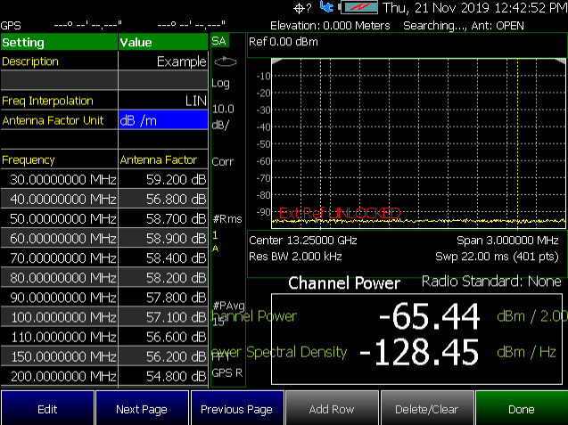
Editing Cable Correction Factors and Adding New Cable Factors
This section contains two procedures illustrating how to edit the Cable Factors settings table values. If New is selected under the X, Y, or Z Antenna or Cable softkey menu, whatever antenna or cable factors that have been imported as the default values and are displayed in the Settings table
1.Selecting an cable softkey menu:
Press Scale/Amptd > More > Corrections then choose one of these softkey menus:
—Cable Off – to open a softkey menu to edit the cable factors for an antenna setup.
2.For this example, the Cable Off softkey menu has been selected:
a.Then press Cable Off > Edit Cable to edit the existing cable’s Frequency and Cable Loss table values that are stored in the FieldFox [:Internal]:\Cable\ directory (Refer to Figure 9-32). Then you can edit the following:
—Description – edits the name of the current cable correction settings table
—Frequency Interpolation – sets the frequency interpolation to linear or to log.
—Frequency – edits the frequency value measured that corresponds to a particular Cable Loss.
—Cable Loss – edits the Cable Loss value that corresponds to a particular frequency.
Refer to next step for details on editing the cable Settings table.
b.Use the arrows, the rotary knob, or numeric keypad to select the table cell value to be edited (i.e., the Frequency Interpolation value is not editable). Then:
—Press Edit Cable to edit your existing cable loss data or
press New to add a a new antenna’s factors or to write over your existing antenna’s file (i.e., Overwrite existing Cable data? is displayed above the table).
—Choose Yes to write over the existing cable file.
—Choose No to create a new cable file (default filename is Example).
—Press Add Row to create additional Frequency and Cable Loss values.
—Press Delete/Clear then choose one of these:
—Delete Row – when pressed this choice deletes the currently selected row of Frequency and Cable Loss (i.e., you must press Yes to delete a row or No to exit the current softkey menu).
—Clear All – when pressed this choice deletes all of the currently selected rows of Frequency and Cable Loss (i.e., you must press Yes to deleted the rows or No to exit the current softkey menu).
—Back – To exit to previous softkey menu.
—Press Done when finished editing to exit.
c.Press Save Cable to save your changes. See also Chapter , “File Saving Naming Options” and then to “Alpha Numeric Editing” on page 879.
For more information:
—See also “GNSS (GPS+) and GPS” on page 886.
Figure 9-33 Example: Editing and Adding a New X axis antenna is shown. But, the Cable Loss table is similar.
Spectrum Emission Mask (SEM) — (SA Mode Only)
This section explains how to make the spectrum emission mask, (SEM), measurement. SEM compares the total power level within the defined carrier bandwidth and offset channels on both sides of the carrier frequency, to levels allowed by standard. Results of the measurement of each offset segment can be viewed separately.
Purpose
The Spectrum Emission Mask measurement includes the in-band and out-of-band spurious emissions. It is the power contained in a specified frequency bandwidth at certain offsets relative to the total carrier power. It may also be expressed as a ratio of power spectral densities between the carrier and the specified offset frequency band.
The spectrum emission mask measurement is a composite measurement of out-of-channel emissions, combining both in-band and out-of-band specifications. It provides useful figures-of-merit for the spectral regrowth and emissions produced by components and circuit blocks.
Measurement Method
The spectrum emission mask measurement measures spurious signal levels in up to 8 pairs of offset/region frequencies and relates them to the carrier power.
The integration bandwidth method is used to perform a data acquisition. The reference channel integration bandwidth (Meas BW) is analyzed using the user defined resolution bandwidth (Res BW), which is much narrower than the channel bandwidth. The measurement computes an average power of the channel or offset/region over a specified number of data acquisitions, automatically compensating for resolution bandwidth and noise bandwidth.
This measurement requires the user to specify the measurement bandwidths of carrier channel and each of the offset/region frequency pairs up to 12 (A - L). Each pair may be defined with unique measurement bandwidths. The results are displayed both as relative power in dBc and as absolute power in dBm.
Summary
Similar to other Radio Channel measurements, SEM sweeps and measures the total power within a Reference channel. It also optionally performs sweeps of user defined offset segments both above and below the reference channel. The peak signals within the offsets are compared against limits, to determine PASS or FAIL results. Tabular data is presented showing individual offset segment results, one row for each offset. A final trace is displayed that contains all of offset segment sweeps and the reference channel sweep is formed and plotted along with the limits.
The following are displayed:
—Total Power Ref (dBm / Hz) - measures total power over the specified Integrated BW.
—Spectrum Emission Mask Pass/Fail – A PASS indicates the displayed SEM is within the current boundaries specified. A FAIL indicates the current signal fails with the specified parameters.
Figure 9-34 SEM Example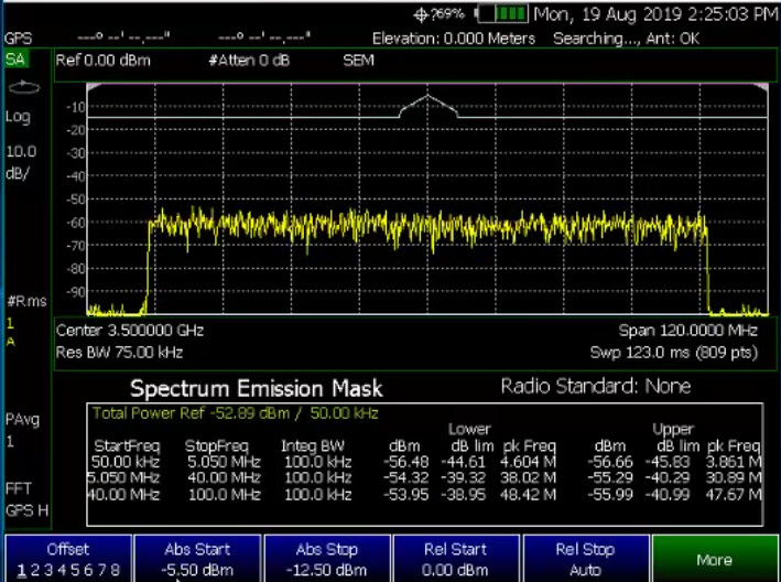
Figure 9-35 SEM Example FAIL Data - Absolute Limit (Blue), Relative Limit (Violet), Trace (Yellow), and Tabular Data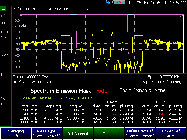
How to select Spectrum Emission Mask (SEM) Measurement
—Press Measure 1 > Channel Measurements > Spectrum Emission Mask
When SEM is selected, the following settings are maintained from a previous measurement: Center Frequency, Preamp ON|OFF, and RF Attenuation.
Setting up the FieldFox for Spectrum Emission Mask (SEM) Measurement
1.Press Measure 1 > Channel Measurements > Spectrum Emission Mask
2.Press Meas Setup 4 then optionally select:
—Averaging Enable/disables averaging and sets the number of trace averages (Default == OFF).
—Meas Type Then select one of the following:
Measurement Type (Meas Type) enables the user to select the method used to calculate the reference power level.
| The displayed green power (dBm)/frequency (Hz) text changes as the Meas Type is toggled |
—Total Pwr Ref (Default == Total Pwr Ref) is the total integrated reference channel power (dBm) is measured and used as the Auto Power Ref value. Peaks found in Offset segments remain in (dBm) units for direct comparison with (dBm) limits.
—PSD Ref the power spectral density (dBm/Hz) is measured and used as the Auto Power Ref value. Absolute Limits and Peaks found in Offset segments are normalized to their equivalent PSD value (dBm/Hz).
—Spec Pk Ref the spectral peak value measured within the reference channel (dBm) is used as the Auto Power Ref value. Peaks found in Offset segments remain in (dBm) units for direct comparison with (dBm) limits. Values in the table are compared to the peak power of the spectrum.
—Ref Channel Opens the Reference Channel softkey menu. Then select one of the following:
—Integ BW Sets the Integrated bandwidth.
—Ref Chan Span Sets the reference channel span. usually set equal or greater than the Integ BW, it is simply a way to reserve additional freq range to be measured for display presentation, if that range is not overlapped by the offset regions. The reference channel is always measured completely as specified, but only the central part of the reference channel that is NOT overlapped by active offset regions is displayed. (Minimum == 10 Hz/ Maximum == Value varies with model and options).
—Carrier Center Tracks currently displayed carrier center frequency (Default == TrackCF). Set to Hold to disable the carrier frequency tracking.
—Res BW Auto/Manual (Default == Auto). Sets the resolution bandwidth. See also, “Resolution Bandwidth (Res BW)” on page 197.
—Offsets Opens the frequency Offsets softkey menu. Then select one of the following:
—Offset Sets the number of pairs of frequencies to be offset (up to eight pairs can be selected).
—Ofst Enable Enables/disables the currently selected Frequency Start/Stop Offset values.
—Ofst Freq Start Sets the offset frequency start value. (Default/Maximum == Value varies with model and options, Minimum == 0 Hz).
—Ofst Freq Stop Sets the offset frequency stop value. (Default/Maximum == Value varies with model and options, Minimum == 0 Hz).
—Res BW Auto/Manual (Default == Auto). Sets the current resolution bandwidth value. See also, “Resolution Bandwidth (Res BW)” on page 197.
—Offset Side Neg Both Pos (Default == Both). Sets the offset side measurement value. Select Negative (Neg) to measure the negative side of the spectrum. Select Positive to measure the positive side of the spectrum.
—Offset Freq Def then select one of the following:
—Carrier Center (Default) applies the frequency offsets to the current carrier center frequency.
—Carrier Edge Selects the edge of the carrier for frequency offset definition.
—Power Ref – the reference power value can be fixed (which also fixes the Relative Limit line), but the user must then consider the unit being used (dBm or dBm/Hz) depending on the Meas Type selected. If Power Ref is left AUTO (Default) then its value will track the Meas Type and change units automatically. Both fixed and Auto settings display the power reference value measured.
3.Setting Center Frequency and Span
| Frequency control menu (Center and Span) provides an SEM Auto Span control (defaulted to ON) which automatically tracks the necessary span to cover all enabled offset segments. In the example in Figure 9-35 on page 258, the necessary span is 16 MHz. But the you can de-couple the span simply by narrowing or widening Span it in order to zoom. The Carrier Frequency (Ref Channel Center) by default tracks the specified Center Frequency, but can be forced to “Hold” at a particular location which would then allow the user Center Frequency to pan above or below for reasons similar to zooming with span. |
Press Freq/Dist then
—Center - sets the center frequency.
—SEM Auto Span - Enables/disables the SEM Auto Span.
—Freq Span - sets the frequency span of the SEM measurement.
—More - optional to set Radio Standard controls. Refer to “Radio Standard” on page 161.
4.Setting the Limit Lines
Two Limit traces are available, an Absolute Limit and a Relative Limit. Both are defined and applied only over the Offset measurement regions. There is no Limit definition or application for the Reference Channel itself. The final Limit Trace displayed is a concatenation of all the individual Offset Limit segments, just as the final measurement trace is. Success or Failure is determined by Fail Mask per offset, to be based on either Relative or Absolute limits, Both (Abs AND Rel), or Either (Abs OR Rel).
Press Limit 8 then
—Offset - selects the offset region to be edited.
The Limits per offset are determined by Start/Stop Amplitude level endpoints, which correspond exactly to the user specified Start/Stop frequency locations in the Offsets sub-menu. So each offset segment is a LINE defined by its two endpoints. In the Limit “Auto” means to match the Start limit value, hence creating a FLAT (horizontal) Limit Line segment. But the Stop value can be manually set as well, creating sloped Limit segments.
—Abs Start - Sets the start of an absolute limit line segment.
—Abs Stop - Sets the stop of an absolute limit line segment.
—Rel Start - Sets the amplitude limit at the start frequency of the offset, relative to the reference power level. The reference power level is displayed in green. The reference power level type can be selected through Measure 1 > Meas Type, and the reference power settings defined through Meas Setup > Ref Channel. Example: If the reference power level reads -15 dBm, and Rel Start is set to -10 dB, the level is -25 dBm. Since this limit line type is relative, it moves with the reference power reading.
—Rel Stop Auto - Sets the amplitude limit at the stop frequency of the offset, relative to the reference power level.
—Fail Mask - Sets the Fail Mask offset parameters for the measurement. Then choose:
—Absolute - The absolute mask is tested for all offsets.
—Relative - The relative mask is tested for all offsets.
—Abs OR Rel - Either Absolute or Relative data failure generates a fail message.
—Abs AND Rel - Requires a relative and an absolute data failure to generate a fail message.
5.Setting the Detectors
The Trace menu shows that two Detector controls are available, one for the Reference Channel (default Auto is Average to facilitate the Power Integration), and another for all the Offset segments (default Auto is PEAK, to facilitate finding PEAK signal energy when comparing against Limits). There is only 1 Trace available, and like the other Channel Measurements, it is set to average.
Press Trace 6 then
—State - sets the measurement state. Refer to “Trace Display States (SA mode)” on page 213.
—Default All - Sets the SEM settings to default
—Chan Detector - Sets the Reference Channel detector (default Auto is Average to facilitate the Power Integration). See also “Detection Method” on page 215.
—Offset Detector - Sets all of the Offset segments (default Auto is Peak, to facilitate finding peak signal energy when comparing against the Limits). See also “Detection Method” on page 215.
—Record Playback - Refer to “Record/Playback (SA Option)” on page 590.
IQ Analysis Streaming (SA Mode Only)
This feature’s intended use is that streamed data is sent to another computer. That computer or another one will act as a SCPI controller and can be used to configure network settings and start or stop streaming. On D-series FieldFox models, streaming can also be configured and controlled from the front panel GUI.
Wideband IQ Streaming enables continuous streaming or recording of IQ data for D-series FieldFox analyzers. The feature supports higher streaming bandwidths, optional 10G Ethernet (SFP+) connectivity, and gap-free operation when used with supported hardware and licenses.
IMPORTANT! - IQ Streaming is used by configuring the desired setup and then starting the acquisition/data stream. In order to make measurement changes (bandwidth, center frequency, etcetera) streaming must be stopped, the new setup configured, and then streaming restarted. - During streaming, the data displayed on the FieldFox is not updated. During streaming, front panel control may be limited. Press Esc to stop streaming. - Streaming to the 10G port (SFP+ port) may stop automatically during power or thermal protection conditions. - FieldFox implements VITA 49, a subset of the VITA 49.2 protocol. Supported sample formats depending on selected protocol and streaming mode. - IQ Streaming uses UDP networking of a 10G Ethernet module. TCP is not supported. - Data for both protocols is 2 floating point values per sample (I and Q). - While in any IQ Analysis mode, the sample rate to frequency span will stay locked/coupled in a ratio of 1.25:1.
|
How to Select IQ Analysis
—In SA mode, press Meas Setup 4
—Then IQ Analysis then choose from
—None – to disable IQ Analysis feature.
—General – to capture IQ data during a measurement. The instrument controls the acquisition process, and the captured data is then processed or stored for further analysis.
—Streaming – to emit a sequence of packets from a specific location in a VRT (VITA 49) enabled architecture (e.g., VRT packet class with a defined packet attribute used in one or more places in an architecture to create packet streams).
When IQ Analysis is selected, the following settings are maintained from a previous measurement: Center Frequency, Span, BW, Sample Rate, Preamp ON|OFF, and RF Attenuation.
How to Setup IQ Analysis General
General setup for IQ Analysis:
1.Press Meas Setup 4 > IQ Analysis > General
2.Press Back to return to the previous softkey menu.
3.Press IQE Sample Rate > Auto (default).
4.Press Average Count > 10 (default). Learn more refer to “Adjusting the Measurement Setup Settings” on page 328.
5.Press Average Type > Auto (default). Learn more refer to “Adjusting the Measurement Setup Settings” on page 328.
6.Press Freq/Dist > Center > 1 GHz
7.Press Freq Span > 1 MHz (default).
IQ Streaming Overview
IQ Streaming allows FieldFox to stream or record continuous I/Q sample data for use with external signal analysis and processing applications. IQ Streaming is an IQ Analysis measurement available in SA mode and can be configured from either the FieldFox user interface or remotely using SCPI commands.
D-Series FieldFox analyzers support wideband IQ Streaming and IQ Recording over 1G Ethernet, 10G Ethernet, or to local storage devices. Depending on installed licenses, hardware, and selected sample format, the analyzer supports gap-free streaming or recording bandwidths up to 40 MHz, with Enhanced mode IQ Streaming supporting up to 120 MHz when using the optional 10G Ethernet interface (lan1). Supported formats include VITA 49, DIFI, and Decodio.
How to Setup IQ Analysis Streaming (Requires Option 351 IQ Analyzer and 353 IQ Streaming, SA Mode Only)
The feature provides continuous streaming or recording of IQ data over supported interfaces.
Wideband IQ Streaming enables gap-free IQ data streaming and recording on D-series FieldFox analyzers. Maximum streaming bandwidth depends on the installed licenses and hardware configuration. Refer to Table 9-1. Table 9-1 IQ Streaming Capability Capability Installed Bandwidth License Maximum Streaming / Recording Bandwidth Standard IQ Streaming Standard bandwidth license Up to 10 MHz. Wideband IQ Streaming Option B04 bandwidth license Up to 40 MHz. Enhanced Wideband IQ Streaming Option B10 bandwidth license with Enhanced mode IQ streaming Wideband IQ streaming (no Recording) gap-free will be supported up to 120 MHz.
Required license:
—Option 351 IQ Analyzer
—Option 353 IQ Streaming
Supported connection types:
—1G Ethernet streaming
—10G Ethernet (SFP+)
—FileSystem recording
If locked to GPS, will populate the timestamp applied to streamed data packets. If not locked to GPS, the system clock time is used to stamp the streamed data packets. Refer to Chapter 31, “System Settings” and to “Frequency Reference” on page 878.
General setup for IQ Streaming and IQ Recording
1.In SA mode, press Meas Setup 4 > IQ Analysis > Streaming
2.Press Settings then:
—Connection Type and choose one of the following:
—1G Ethernet - Sets IQ Streaming through the LAN port using a 1G Ethernet connection.
—10G Eth. (SFP+) - Sets IQ Streaming through the SFP+ port using a 10G Ethernet connection.
—FileSystem - Sets as IQ recording.
When the Connection Type is set to 1G or 10G Ethernet (IQ streaming), configure the following settings.
—Dest LAN IP - Click and select Other... to enter new IP address of the destination host.
—Dest Port - Change the default UDP socket 4991.
—Enhanced Mode - This softkey available only when the Connection Type is set to 10G Ethernet.
—ON - Enables high-bandwidth IQ Streaming over the optional 10G Ethernet interface. Supports streaming bandwidths of up to 120 MHz, depending on the installed license, hardware configuration and selected sample format (VITA 49 or DIFI).
—OFF (default) - Selects standard IQ Streaming or IQ Recording operation. Supports streaming bandwidths of up to 40 MHz, depending on the installed license, hardware configuration and selected sample format (VITA 49 or Decodio). VITA 49 is the only protocol available for IQ Recording.
When the Connection Type is set to FileSystem (IQ recording), configure the following settings.
—Press Recording Settings to configure IQ recording.
a.Device - Select the appropriate storage location for the IQ recording.
—USB - An external USB flash drive (must be inserted).
For best performance, use a USB SuperSpeed storage device. High-performance USB SSD or USB-C NVMe storage devices may be required to achieve gap-free recording bandwidths up to 40 MHz and maximize recording throughput.
—Internal - FieldFox memory.
—SD Card - An external SD Card (must be inserted).
Recorded files are stored in the IQRecording folder on the selected device. IQ Recording files are saved in VITA49A format (*.vita49).
b.Rec Duration - Specify a Recording Duration in second (s), minute (min) or hour (hr).
c.Recording Name - To set the recording name in the recording File dialog.
The recording will first be assigned an automatic filename.
d.Manage Recordings - To edit the recording filename or delete old recordings.
e.File Format - To select IQ recording file format. Currently only support VITA 49 format.
3.Press Meas Setup 4 > IQE SampRate > Manual > 1.25 MHz (default when set to Auto).
Setting the IQE sample rate to Manual, forces the Span to be: The IQE Sample Rate and Frequency Span settings are coupled. Adjusting either parameter automatically updates the other to maintain the required sample rate-to-span ratio of 1.25:1.
Span = 0.8 * Sample rate.
4.Configure Center Frequency, and Span
a.Press Freq/Dist > Center > 1 GHz
b.Press Freq Span > 1 MHz (default).
This forces the Sample rate to be:
Sample rate = 1.25 * Span.
5.Adjust receiver gain if desired. Configure Ref Level, Preamp, and RF Attenuation. Typically, the goal is to be able to see the desired signal that you want to capture as close as possible to the top of the display grid on the screen, without causing an ADC over range to be displayed. This maximizes the signal-to-noise ratio.
Press Scale/Amptd then
—To configure automatically: Press Ref Level – adjust as needed.
or
To adjust manually:
—Press Preamp ON (Default == OFF)
—Press RF Atten > Manual > 15 dB (default)
6.Press Protocol Settings To configure IQ Streaming protocol:
—Protocol - Specifies the data format used to stream or record IQ data. Three streaming protocols are supported.
—VITA49 - Streams or records I/Q data using the VITA 49 standard format. VITA49A is the only protocol supported for IQ Recording, which is available only in Standard IQ Streaming mode. For IQ Streaming, VITA49A is supported in both Standard and Enhanced IQ Streaming modes. For information on analyzing VITA 49 streams or VITA 49 recording files using Keysight 89600 VSA software, refer to Chapter 18, “Remote Server Mode (Requires SA Option 233)”.
—Decodio - Streams I/Q data using the Decodio format for compatible analysis applications. Available only in standard IQ Streaming mode.
—DIFI - Streams I/Q data using the Digital IF Interoperability (DIFI) standard for Enhanced IQ Streaming applications. Available only in Enhanced IQ Streaming mode. —DIFI is available only when Enhanced Mode is enabled. —DIFI supports only 8-bit Fixed and 16-bit Fixed sample formats. —Decodio is available only when Enhanced Mode is disabled. —Decodio supports only 32-bit Float sample format. —VITA 49 is available in both Standard and Enhanced modes. —VITA 49 supports all 8-bit Fixed, 16-bit Fixed, and 32-bit Float sample format. —32-bit Float sample format is not supported in Enhanced mode. When Ethernet media is selected, streaming transmits UDP packets using the selected protocol.
When Filesystem media is selected, the same packets will be stored to a file instead.
—Context Rate - Not available when the Decodio protocol is selected. Specifies the frequency of context packet generation. A setting of zero for Context Rate generates one context packet at the start of the streaming session and no additional context packets thereafter.
—Vita Stream ID - Not available when the Decodio protocol is selected. Used to distinguish between multiple IQ streams received by the receiver.
—Packet Size - Setting the number of samples per packet.
—Auto (Default) - Automatically selects an appropriate packet size (samples per packet).
—Manual - To specify the packet size. When streaming to Ethernet, packet size is limited to 9000 bytes when Allow Fragment is Off, and 64 KB (maximum UDP packet size) when Allow Fragment is On. When recording to disk, the maximum packet size is 256 KB due to VITA 49 and VSA limits.
—Sample Format - Specifies the data type and resolution used for I and Q samples during streaming or recording. Refer “Protocol Restriction”, on page 268 for the sample format restriction.
—16 bit Fixed - Optimal format (Recommended).
—32 bit Float - Higher dynamic range.
—8 bit Fixed - Higher throughput with trade off dynamic range. Supported Sample Formats by IQ Streaming Protocol: —VITA 49: All sample formats are supported. —DIFI: Only 8-bit and 16-bit data formats are supported. —Decodio: Only the 32-bit Float sample format is supported. —Enhanced Mode: The 32-bit Float sample format is not supported.
—Allow Fragment - Not supported for the Enhanced mode IQ Streaming. Enables or disables IP packet fragmentation during Ethernet IQ streaming, allowing to set a packet size larger than the configured MTU limit.
—ON - Enables packet fragmentation.
—OFF - Disables packet fragmentation. Allow Fragment available for VITA 49 and Decodio protocols. Allows setting a packet size larger than the MTU limit.
—More - Appear only when DIFI protocol is selected or Enhanced IQ Streaming is enabled. Provides access to additional DIFI protocol settings and the VITA 49 ARP Refresh setting.
—Reference Point - Specifies the signal reference point reported in the DIFI stream metadata. Choose from
——RF Output - Uses the RF output connection as the reference point.
——Analog IF - Uses the Analog IF signal path as the reference point.
——Antenna Feed - Uses the antenna input connection as the reference point.
—IF Ref Freq - Sets the IF reference frequency included in the DIFI stream metadata.
—RF Ref Freq - Sets the RF reference frequency included in the DIFI stream metadata.
—IF Band Offset - Sets the frequency offset between the RF center frequency and the digital IF bandwidth center used in the DIFI stream.
—ARP Refresh - Sets the ARP refresh interval used to maintain network connectivity during IQ Streaming.
7.Press Start Streaming - Start IQ Streaming or start recording to a file.
8.When done press Esc to stop streaming or stop recording. When recording to file, the recording automatically stops after the set duration (in seconds) has elapsed.
Or via the FieldFox front panel, choose:
—Press Meas Setup 4 > IQ Analysis > None
Or simply choose:
—Press Measure 1 > All Meas Off
For IQ Streaming SCPI command refer to the FieldFox Programming Guide: https://helpfiles.keysight.com/csg/FFProgrammingHelpWebHelp/A_SA_Mode_Commands.htm
Effective Isotropic Radiated Power (EIRP) – (SA Mode Only)
How to Select Effective Isotropic Radiated Power (EIRP)
1.In SA mode, press Measure 1
2.Then Channel Measurements > Channel Power > EIRP Off to open a menu of softkeys to set up EIRP.
How to Setup EIRP (Effective Isotropic Radiated Power)
General setup and an example for EIRP:
For this example we are using an isotropic antenna with the following specifications:
—Frequency range: 9 kHz to 9 GHz isotropic antenna
—Preamp stages: 2 (+15 dB each (@2 GHz)
—Chop/Switch speed rate: 1 Hz to 50 kHz
—Assume: 600 Series 50ꭥ coaxial cable with 2.5 dB/100 feet
1.Press Measure 1 > Channel Measurements > Channel Power > EIRP Off then choose from the following:
—EIRP Meas OFF ON – Enables and disables the EIRP measurement.
—Rx Ant Gain – Enter the receiver ant gain (–100 dB to 100 dB; Default == 0 dB).
For this example: 30 dB > Enter.
—Dist to Ant – Enter the distance between the receiving and transmitting antennas (0 m to 25 km; Default == 100m)
For this example: 100m (default)
—Rx Cable Loss – Enter the receiver cable loss (0 to –100 dB; Default == 0 dB).
For this example: 2.5 dB
—Margin Comp – Enter the margin compensation to remove known self-interference, antenna efficiency, fading and other errors (–100 dB to 100 dB; Default == 0 dB).
—Then More and choose from the following:
—Restart – Press this softkey to restart an antenna measurement.
—Save Horizontal – Saves the current horizontal EIRP value (dBm).
—Save Vertical – Saves the current vertical EIRP value (dBm).
—Clear H & V –Clears the saved horizontal and vertical EIRP values (dBm).
2.Configure Center frequency, Span, Preamp, and RF Attenuation
—Press Freq/Dist > Center > 2 GHz
—Press Freq Span > 3 MHz (default)
—Press Scale Amptd > Preamp > ON (Default == OFF)
—Press RF Atten Auto (Default == Auto)
3.Summary of EIRP setup, per step 1.
—Press Rx Ant Gain For this example: 30 dB > Enter.
—Press Dist to Ant For this example: 100m (default)
—Press Rx Cable Loss For this example: 2.5 dB
—Press Margin Comp
4.Start EIRP: Press Restart
5.When done press:
Save Horizontal and
Save Vertical
6.Optional: To clear the saved horizontal and vertical EIRP values press:
Clear H & V