Analyzing Transmission Line (RLCG) Parameters

Note: Your PLTS application may not include the optional RLCG analysis feature.

Overview

There are four modes in which RLCG parameters may be displayed in PLTS:

W-Element
Differential
Common
Self/Mutual

PLTS exports RLCG data in the W-Element mode for use by HSPICE or Advanced Design System (ADS - an integrated design software and test instrumentation solution from Keysight Technologies). The W-Element mode uses the 4-port S-parameters of the symmetrical, coupled transmission line to compute the R (resistance), L (inductance), C (capacitance), and G (conductance) parameters. Each is displayed in a 2-by-2 matrix. There is an R-value for each line and coupling values for R. The same is true for L, C, and G. These parameters can then be used in HSPICE or ADS as a model of the measured transmission line.

There are two modes, Differential and Common, of the RLCG parameters that treat the coupled line as a 2-port device instead of a 4-port device. These modes simply use the four pure differential-mode parameters or four pure common-mode parameters as a 2-port S-parameter device. This is saying we have a line driven differentially (or in common) and what are the RLCG parameters, impedance, and propagation constant for this line. In this case, the RLCG parameters are a single value, not a 2-by-2 array. There is no self or coupling since it is treated as a single line. Neither of these modes is directly usable in HSPICE or ADS but these modes can give insight to an experienced user.

The fourth mode is the Self/Mutual mode. It is a slight deviation from the W-Element mode. The only difference in this mode is the way that the coupling between parameters is defined. The conversion is described in CPTL RLCG Extraction Procedure.

An important issue that is not clearly understood is that the measurements must be for only the line to be modeled. Connectors and single-ended launches to connect to the actual coupled line must be removed using de-embedding or calibration standards in the media. The simplest way to measure coupled lines is by probing the lines. When the lines are probed, no connectors or launches need be removed.

Note: When extracting the RLCG parameters for a symmetrical coupled line, the measurement must include only the coupled transmission line. It should not include any connectors, or single-ended launches in the measurement. If any of these are included, the parameters will not accurately model the transmission line. Refer to Considerations When Extracting RLCG Parameters for more information. Note that the following image shows the connector and launches that need to be removed.

Transmission Line Parameters

Transmission lines are distributed devices. However, SPICE type simulators work with lumped elements, not distributed elements. RLCG type models are commonly used to approximate the distributed behavior of a transmission line. The single transmission line shown below can be modeled by a network consisting of a series resistance and inductance with parallel capacitance and conductance.

Note: It should be clearly noted that the PLTS RLCG tool is designed specifically for differential (not single-ended) transmissions lines with the following characteristics:

The main application for PLTS RLCG is for scalable models on interconnect where the PCB trace cross section geometry is constant. For example: same dielectric thickness, trace width, trace thickness, foil thickness, etc. This allows for various length backplane channels to be generated from one RLCG model. Input the length, then the RLCG model is automatically generated for self and mutual reactance figures of merit for each length of backplane trace. Note that no backplane connectors are included.
If a 2-port file is imported into PLTS then RLCG is selected, the following error message is displayed:
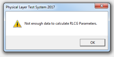
PLTS RLCG analysis is only for constant impedance lines with no discontinuities (like on connector vias). If there is a complex impedance profile like on most high speed digital channels with connectors, this version of RLCG modeling is not useful.

RLCG Model for Single Transmission Line

The different terms included in the model describe the following physical phenomena:
R	Resistive loss of the conductor (transmission line trace). Determined by the conductance of the metal, width, height, and length of the conductor.
L	Inductive part of the circuit resulting from the layout of the conductors. Determined by the dimensions of the conductor, permeability of the metal, and layout.
C	Capacitive part of the circuit resulting from the layout of the conductors. Determined by the permittivity and thickness of the board material and the area of the conductor.
G	Shunt loss of the dielectric. Determined by the layout of the conductors, permittivity, loss tangent and thickness of the board material.

RLCG modes are frequency-based models

The following image shows the attenuation from Copper Loss and Dielectric Loss.

Equation Set 1 describes the most adopted frequency dependencies of RLCG parameters.

Equation
Set 1

R = RDC+RSKIN √F

L = constant

G = GDC + GAC x F

C = constant

Note: These parameters are called fitted parameters.

The values for RLCG are typically specified in per unit length, where the unit of length is in meters. Therefore for a given length of line the value for each of the parameters is easily determined. To best approximate the distributed behavior of the transmission line multiple sections of RLCG circuits are used. The value of the parameters, R for example, is determined by dividing the R value for the given length of line by the number of sections. Since R (and) L values add in series and C and G values add in parallel, a multi-section model for simulation can easily be constructed. For example:

If the value of R for a given line is 2.4 ohms per meter,

and the length of line needed is 100 cm,

then the total resistance needed for the 100 cm line is 0.24 ohms.

If 12 sections are used to model the line, then each R is 0.02 ohms.

The same calculation can be made for each of the parameters.

Extracting Fitted RLCG Parameters from S-Parameters

Telegrapher's equations are used to solve for the RLCG values. The Telegrapher's equations described in Coupled-Transmission Line Models for the 2-coupled line model. Telegrapher's equations deal with the voltage and current as shown earlier. However, PLTS measures S-parameters, which are ratios of power reflected from and transmitted thru to the incident power. For a single transmission line, the impedance (Z) and propagation constant (g) can be derived from the measured 2-port S-parameters of the line. Equation Set 2 defines the S-parameters in terms of Z, Z0 (characteristic impedance of the measurement system), g, and l (the length of the line).

Equation Set 2

where

Using Equation Set 2 and transforming to [ABCD} parameter, we can solve for g and Z as functions of S-parameters as shown in Equation Set 3 and Equation Set 4:

Equation
Set 3

where

Equation
Set 4

Once g and Z are known, from the standard transmission line relationships, values for R, L, C, and G can be determined as shown in Equation Set 5 through Equation Set 10 below:

Equation
Set 5

Equation
Set 6

Then,

Equation
Set 7

Equation
Set 8

Equation
Set 9

Equation
Set 10

In the case of a pair of coupled transmission lines, each RLCG parameter is actually a 2-by-2 matrix. For symmetrical uniform coupled transmission lines, the matrices are real and symmetrical. The latter is described in more detail in Coupled-Transmission Line Models.

Coupled-Transmission Line Models

Start with an ideal lossless symmetrical coupled-transmission line (CPTL):

The Telegraphers set of equations are described below:

Equation
Set 11

Equation
Set 12

These equations represent the closest form to the physical behavior of CPTL, since they describe each line by its own self parameters (L and C) and the different mutual couplings (Lm and Cm). Obviously, these equations can be extended for the lossy case, where the conductor and dielectric losses would be taken into account.

Note: These parameters are called self-parameters.

By rearranging Equation Set 11 and Equation Set 12, a second set of parameters can be defined as shown in Equation Set 13 and Equation Set 14:

Equation
Set 13

Equation
Set 14

In the general case, RLCG parameters are grouped in 2-by-2 real matrices, each term being frequency-dependent. In the case of symmetrical coupled-lines, these matrices are symmetrical. See Equation Set 15.

Equation
Set 15

Note: These parameters are called spice-parameters.

Most Spice-type simulators use this type of model description with different variations in the implementation. This aspect is described in more details in Importing and Exporting Data.

The third model representation is called the Differential-Common Modes Equivalent Model. This model was created because the RLCG extraction algorithm deals only with Single-Ended Transmission Lines (SETL). See Extracting Fitted RLCG Parameters from S-Parameters. Therefore, each quadrant from the mixed-mode S-parameters, in particular the Diff-Diff and Com-Com, are treated as two separate SETL, with predefined normalized impedance.

The new set of RLCG parameters extracted for the differential and common modes can be represented in a frequency-dependent matrix format, as shown in Equation Set 16.

Equation
Set 16

Note: These parameters are called Diff/Com parameters.

CPTL RLCG Extraction Procedure

PLTS starts by extracting the RLCG parameters for both the Diff-Diff mode and the Com-Com mode. In the case of a symmetrical CPTL, mode-conversion should be negligible. Then we offer the following options to visualize.

This section describes the formulas for the different transformations.

Equation Set 17 and Equation Set 18 relate the Odd and Even modes to the Differential and Common modes of propagation:

Equation
Set 17

Equation
Set 18

Using the propagation constant and the characteristic impedance for the Odd/Even modes, the Spice parameters are derived in Equation Set 19 and Equation Set 20.

Equation
Set 19

Equation
Set 20

Finally, Self parameters can be derived as shown in Equation Set 21 and Equation Set 22.

Equation
Set 21

Equation
Set 22

RLCG Output Plots

The following illustrates the difference between the extracted parameters and the fitted curve.

This plot format can be applied to Diff/Com, Spice or Self parameters.

The following illustrates the propagation constant and the image after that illustrates the characteristic impedance in real-imaginary format. Since these two parameters are complex numbers, you have the choice of plotting these parameters in other formats, like Magnitude/Phase, and dB/Phase versus linear or log of the frequency.

Impedance versus Frequency

Considerations When Extracting RLCG Parameters

When extracting the RLCG parameters for a symmetrical coupled line, the measurement must include only the coupled transmission line. It should not include any connectors, or single-ended launches in the measurement. If any of these are included, the parameters will not accurately model the transmission line. The following shows the connector and launches that need to be removed.

The effects to the left of the dotted line need to be removed. These can be removed one of two ways. The first is to characterize the launch structure (to the left of the dotted line) and then de-embed it from the measurement. This is not easily done. The other way is to create calibration standards on the board that include the connector and launch and use them to calibrate with. However, the parasitics of the standards need to be characterized and entered into the calibration kit definition.

The easiest way to characterize the transmission line is to do a probed measurement. By performing a probe calibration there are no connectors or launches to remove. The following shows a typical probed measurement.

The Parameters for Each RLCG Mode

The data (parameters) available for each of the four RLCG modes varies due to the model assumptions. The individual parameter selections are based on the specific RLCG data analysis type. The following lists each data analysis type and its associated parameters.

RLCG (Differential): Rd, Ld, Cd, Gd, Zor, Zoi, Ad, Bd

RLCG (Common): Rc, Lc, Cc, Gc, Zor, Zoi, Ac, Bc

RLCG (W-Element): R11, L11, C11, G11, R12, L12, C12, G12

RLCG (Self/Mutual): Rs, Ls, Cs, Gs, Rm, Lm, Cm, Gm

where,

A represents the Attenuation Constant (a)

B represents the Phase Constant (b)

C represents Capacitance

G represents Conductance

L represents Inductance

R represents Resistance

Z represents Impedance

Viewing Transmission Line Data

There are eight transmission line parameters for each transmission line mode.

Learn how to open Transmission Line Plot windows

Setting Transmission Line Characteristics

After selecting a RLCG parameter, the T-Line Characteristics dialog box is displayed.

This setting can also be made at any time by clicking Tools, then T-Line Characteristics.

T-Line Characteristics dialog box help

Enter the length of the transmission line (in meters) and the highest measured frequency (in megahertz) and then click OK.

Length (M) can be used to scale extracted values in units/meter.

Highest Extracted Frequency (MHz) defaults to the stop frequency value. However, this can be set at a lower frequency to better fit your parameters.

The highest extracted frequency is 90% of the maximum measured frequency. For example, the Highest Extracted Frequency (MHz) is 45 GHz for a 50 GHz measurement. In the case shown above, the Highest Extracted Frequency (MHz) is 8100 MHz for the 9 GHz measurement. This allows for some guard band of the data, extra bandwidth for use in time to frequency conversions, and to allow some extra frequency range to get good data and allow for time domain roll off.

Viewing RLCG W-Element - Fitted and Smoothed Traces

When data is viewed in RLCG (W-Element), two traces are displayed in each of the eight plots. The two default traces in each plot are the Extracted data (represented by the blue trace) and Fitted data (represented by the red trace).

However, both traces may not be readily apparent in every plot initially. Both R (R11 and R12) and both G (G11 and G12) plots may appear to have only the red Fitted traces. The R plots can easily be resolved by autoscaling both of plots (see Autoscale). For the sloping linear G plots, the red Fitted trace is lying exactly on top of the blue Extracted trace.

In W-Element, viewing the Extracted data with the Fitted data is the default status. However, you have the option of viewing the Extracted data with Smoothed data as well. The following shows W-element plots for R11 and L11 extracted data traces. In addition to the Extracted data traces, the upper two plots also show the default Fitted data traces. In the lower two plots, the Extracted data traces are shown with Smoothed data traces.

Extracted Data

Extracted data is the data that has been derived (or extracted) from the measured frequency domain values. The blue extracted data trace is always displayed in the W-element. This data can also be exported using the RLCG export feature. Learn how.

Fitted Data

Fitted data is used to show the general trend of the extracted data using a minimal set of data. The trend is defined by the W-Element model definitions in HSPICE. It is the traditional lossy transmission model common in most simulators. The fitted data set is computed from the extracted data and used to define each of the traces. Fitted data is displayed with a red trace.

Resistance (R): R has two values for each trace R0 and RS. R varies as the square root of frequency, so R at a given frequency point can be calculated with the formula:
where R0 is the R value at 0 Hertz and RS is the parameter for the frequency variation.
Inductance (L): Each L has one value, which is the average of the extracted data values for L and is constant versus frequency.
Capacitance (C): Like L, each C has one value, which is the average of the extracted data values for C and is constant versus frequency.
Conductance (G): G has two values for each trace G0 and GD, G is linear as a function of frequency, so G at a given frequency point can be calculated with the formula:
where G0 is the G value at 0 Hertz and GD is the slope value.

From these values, each of the fitted traces are calculated and displayed. These values can also be exported using the RLCG export feature. See RLCG.

Smoothed Data

Smoothed data is extracted data that has had a smoothing mask applied making the result display the general trends of the extracted data. As additional points are added to the smoothing mask, more of the extended data's peaks and dips are rounded off (or smoothed). Smoothing uses a running average approach at each data point to smooth the data. For example, if the integer "5" is entered as the smoothing value, at data point N, PLTS averages the five values ( N-2, N-1, N, N+1, N+2) for data point N. This averaging is used for every data point. Smoothed data is displayed as a red trace. This data can also be exported using the RLCG export feature. See RLCG..

To View the W-Element Data with the Smoothed Data Option

From the Tools menu, select W-Element Display Configuration.

Select Smoothed in the Additional W-Element Trace area to view the smoothed data.

In the Number of Points in Smoothing Mask area, enter the number of points for the smoothing mask for the desired parameter. Continue entering the smoothing values for all desired parameters. In this example, the value 501 was entered as the value in the R11 box. The number of point values must be odd integers.

Click Apply.

This dialog box remains displayed so that changes to the point values may be optimized or you may return to viewing the Fitted traces. The Close button closes the dialog box.

TIP As additional points are added to the smoothing mask, more of the extended data's peaks and dips are rounded off (or smoothed). A change in the number of points at the lower end has a more dramatic smoothing effect than a similar change at the higher end. As an example, the change from 51 to 501 points has a greater effect to the trace than from 501 to 1001 points. Refine the number of points so the smoothing traces are displayed to meet your requirements.