FFT Operator
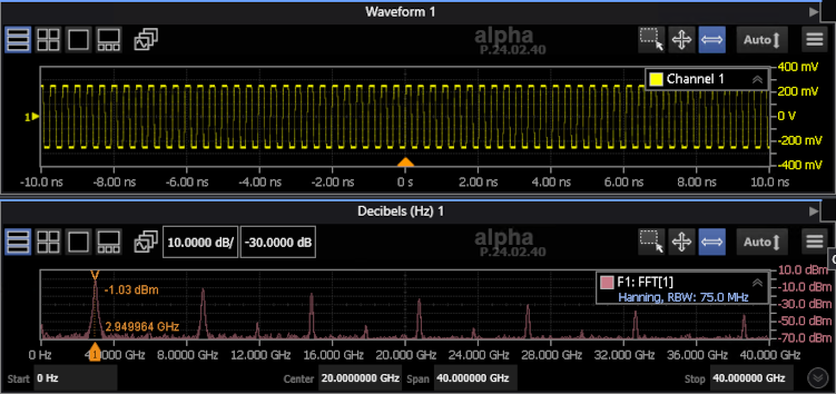
![]() The Fast Fourier Transform (FFT) function takes the sample points of the waveform in the time domain and computes the frequency components.
The Fast Fourier Transform (FFT) function takes the sample points of the waveform in the time domain and computes the frequency components.
After placing the function, click the function icon to open the FFT Operator Setup dialog box.
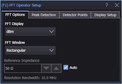
FFT Options
-
FFT Display — Select to display the FFT to be one of the types that is listed in the following table.
FFT Display Shown in
Waveform Content WindowNotes dBm Decibels (Hz) dBV Decibels (Hz) dBmV Decibels (Hz) dB (Normalized) Decibels (Hz) dBm/Hz (NSD) Decibels (Hz) For Noise Spectral Density (NSD) measurements where a constant will be subtracted from the FFT function. Linear Magnitude Waveform Phase Degrees (Hz) Unwrapped Phase Degrees (Hz) Group Delay Seconds (Hz) If Phase, Unwrapped Phase, or Group Delay is selected, the FFT Phase Reference field is displayed, which you can define to be Left, Center, or Manual. Selecting Manual to enter the FFT Origin in seconds.
-
FFT Window — Choose Rectangular, Hanning, Flat Top, Blackman-Harris, or Hamming windows for your FFT function.
Use Hanning or Hamming for best frequency accuracy, Flat Top for best amplitude accuracy, and Rectangular for single-shot transients or signals where there is an integral number of cycles in the time record.
The FFT operation assumes that the time record repeats infinitely. Unless there is an integral number of cycles of the sampled waveform in the record, a discontinuity is created at the end of the record. This is referred to as "leakage". To minimize spectral leakage, windows that approach zero smoothly at the beginning and end of the record can be used as filters for the FFT.
Windows work by weighting points in the middle of the waveform record higher than those at the ends of the record. For example, a Hanning window looks like the first half cycle of a sine wave. The Hanning window multiplies the points at the middle of the record by 1 and multiplies points at the start and end of the record by zero.
-
Reference Impedance — When the vertical Units are displayed (and measured) as power (that is, dBm or Watt), this control lets you specify the reference impedance of the Source so that power is calculated correctly. You can select automatically determined or manually entered values:
-
Auto — When selected, analog input channel reference impedances can be automatically determined by the type of probe detected (differential, common mode, single-ended) or by whether two channels are set up as Differential Channels or Common Mode Channels in the Channel dialog box.
For: The automatically determined Reference Impedance is: Single-ended input channels and almost all high-impedance probes 50 Ω Differential input channels1 and differential probes 100 Ω Common Mode input channels1 and common mode probes2 25 Ω NOTES:
1The Channel dialog box Differential Channels or Common Mode Channels selections take precedence over the detected probe type.
2Common mode is not available on high-impedance probes.All other sources (math functions, waveform memories, etc.) are assumed to be 50 Ω. If this is not correct, for example, when a waveform memory or math function source comes from a differential or common mode signal, you must clear the Auto selection and manually enter the appropriate reference impedance.
-
When Auto is not selected, you can manually enter a reference impedance value from 10 Ω to 200 Ω.
-
-
Resolution Bandwidth (RBW) — The FFT resolution, which is defined as sampling rate / memory depth when using the Rectangular window (other windows have a Normalized Equivalent Noise Bandwidth factor applied). If the sample size is not a power of two number of points, the Infiniium application adds zeros equally to the beginning and end of the data until there is a power of two number of points.
You can adjust the resolution bandwidth by changing the memory depth and/or sampling rate acquisition setup options when they are in manual mode. See Acquisition Tab.
To ensure that enough data is available to construct a useful FFT, set Infiniium's timebase scale equal to the waveform's period. This will display 10 waveform cycles. For example, for a 5 GHz (200 ps) reference clock, enter a scale setting of 200 ps/division.
Tracking markers cannot be positioned between the graph's data points. This will become noticeable as the graph's span is reduced. Dragging the marker or clicking the position arrows in the Marker's dialog box always results in the marker being placed on a data point. If, however, you enter a specific marker position in the dialog box's Position field that is not at a data point, the marker will move to the entered frequency location but the amplitude value will be equal to the amplitude at the nearest sampling point.
See Also
For information on the Peak Detection, Detector Points, and Display Setup tab controls, see:
Content Windows
The FFT waveform is automatically displayed in the appropriate type of content window, which is listed in the following table.
Under remote control, additional content windows of the same type are available which you can optionally move the waveform to using the :FUNCtion{1:64}:CWINdow command.
When you display the FFT as a Linear Magnitude, the waveform is displayed in the Waveform 1 waveform content window (but it can be moved to other Waveform windows).
| FFT Display Selection |
Displayed Content Window |
Number of Available Windows |
Scale Units |
|---|---|---|---|
| dBm | Decibels (Hz) | 4 | Y-Axis: dBm (logarithmic scale) X-Axis: Hertz |
| dBV | Y-Axis: dBV (logarithmic scale) X-Axis: Hertz |
||
| dBmV | Y-Axis: dBmV (logarithmic scale) X-Axis: Hertz |
||
| dB (Normalized) | Y-Axis: dB (logarithmic scale) X-Axis: Hertz |
||
| dBm/Hz (NSD) | Y-Axis: dBm/Hz (logarithmic scale) X-Axis: Hertz |
||
| Linear Magnitude | Waveform | 4 | Y-Axis: Volts or Watts (linear scale) X-Axis: Hertz |
| Phase | Degrees (Hz) | 4 | Y-Axis: phase (°) X-Axis: Hertz |
| Unwrapped Phase | |||
| Group Delay | Seconds (Hz) | 4 | Y-Axis: seconds X-Axis: Hertz |