3CAT (Cable and Antenna Test) Mode
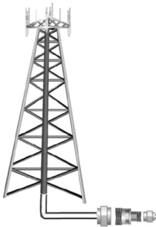
| CAT Mode is typically used to test an entire transmission system, from the transmitter to the antenna. This process is sometimes referred to as Line Sweeping. CAT Mode is similar to NA (Network Analyzer) Mode. Learn more in the Supplemental Online Help: https://rfmw.em.keysight.com/wireless/helpfiles/FieldFoxOnlineSupplementalHelp/Home.htm. CAT Mode Distance to Fault measurements are discussed in Chapter 4, “DTF (Distance to Fault) Measurements.”. |
| IMPORTANT! For CAT and NA modes, limit lines do not apply |
In this Chapter
See Also
Chapter 8, “Calibration for NA, CAT, and VVM Modes”, on page 131 | |
Learn more in Making 75Ω (ohm) Measurements in the Supplemental Online Help at: https://rfmw.em.keysight.com/wireless/helpfiles/FieldFoxOnlineSupplementalHelp/Home.htm. |
Select CAT Mode before making any setting in this chapter.
1.Press Mode.
2.Then CAT/TDR.
How to select a CAT Mode Measurement
Learn more in the Supplemental Online Help at: https://rfmw.em.keysight.com/wireless/helpfiles/FieldFoxOnlineSupplementalHelp/Home.htm.
Press Measure 1.
Then choose one of the following: These softkeys also appear after CAT Mode is selected.
—Distance To Fault 1-port reflection measurement that uses Inverse Fourier Transform (IFT) calculations to determine and display the distance to, and relative size of, a fault or disruption in the transmission line. Units are in return loss format, expressed as a positive number in dB, unless the measurement selected is DTF (VSWR). Learn more about DTF Measurements refer to Chapter 4, “DTF (Distance to Fault) Measurements.”.
—Return Loss & DTF Displays both a Return Loss measurement and a DTF measurement. Use this format to display the frequency settings that are used to make the DTF measurement. The frequency range settings for these two measurements can be coupled or uncoupled. Learn more, “Coupled Frequency” on page 64.
—Calibrations are applied to both traces
—When in Hold mode and Single sweep is performed, only the active trace is triggered. Use the  arrows to activate a trace
—Return Loss 1-port reflection measurement that displays the amount of incident signal energy MINUS the amount of energy that is reflected. The higher the trace is on the screen, the more energy being reflected back to the FieldFox. Learn how to measure Return Loss on “Return Loss Measurements” on page 65.
—VSWR (Voltage Standing Wave Ratio – also known as SWR) 1-port reflection measurement that displays the ratio of the maximum reflected voltage over the minimum reflected voltage. The higher the trace is on the screen, the more energy being reflected back to the FieldFox.
—DTF (VSWR) Distance to Fault in VSWR format.
—Cable Loss (1-Port) 1-port reflection measurement that displays the loss of a transmission line. Learn more, see “1-Port Cable Loss Measurements” on page 66.
—Insertion Loss (2-Port) 2-port transmission measurement that accurately displays the loss through a cable or other device in dB. Both ends of the cable must be connected to the FieldFox. NO phase information is included in this measurement. Learn more, see “2-Port Insertion Loss Measurements” on page 67. This feature is available only with an option on some FieldFox models. For detailed information, please view the FieldFox Configuration Guide at: https://www.keysight.com/us/en/assets/3125-1447/configuration-guides/FieldFox-Handheld-Analyzers-D-models.pdf
—DTF (Lin) Distance to Fault in Linear format.
—TDR (Lin rho) The Y-axis of the display is linear, real, unitless values. A trace without reflections shows as 0 (zero). Maximum reflections from an open or short show as 1.
—TDR (ohm) The Y-axis of the display is impedance (ohms).
—TDR & DTF Both TDR and DTF traces are displayed.
Both CAT and NA Modes allow you to view and change most relevant settings from a single location. All of these settings are discussed in this chapter and, unless otherwise noted, ALL of these settings can also be made using the standard softkey menus.
How to view and change Quick Settings
—Press Meas Setup 4 > Settings.
—Press Next Page and Previous Page to view all settings. If these softkeys are NOT available, then all available settings fit on one page.
—To change a setting:
—Use the arrows to highlight a setting.
—Then press Edit. The current setting changes to yellow.
—Some settings require you to press a softkey to change the value. Otherwise, use the numeric keypad, arrows, or rotary knob to change the value.
—When finished changing a value, press Done Edit.
—Press Dock Window to relocate the Settings table to a position relative to the trace window. The Dock Window setting persists through a Preset. Choose from the following:
—Full (Default setting) Only the Settings table is shown on the screen. The trace window is temporarily not shown
—Left The Settings table is shown to the left of the trace window
—Bottom The Settings table is shown below the trace window
—When finished changing ALL settings, press Done to save your settings
Set the range of frequencies over which you would like to make CAT Mode measurements.
When the frequency range is changed after a calibration is performed, the cal becomes interpolated. Learn more in “Interpolation *” on page 149.
—Press Freq/Dist.
—Then choose from the following
—Start and Stop frequencies - beginning and end of the sweep.
—Center and Span frequencies – the center frequency and span of frequencies (half on either side of center).
—Follow each setting by entering a value using the numeric keypad, arrows , or the rotary knob.
—After using the keypad, select a multiplier key. Learn about multiplier abbreviations in Chapter 1, “Overview.”
—After using the arrows or the rotary knob, press Enter. The amount of frequency increment is based on the current span and can NOT be changed in CAT Mode.
Adjust the Y-axis scale to see the relevant portions of the data trace. The Y-axis is divided into 10 graticules.
This setting can be changed at any time without affecting calibration accuracy.
—Press Scale / Amptd.
—Then choose from the following three methods:
1.Autoscale Automatically adjusts the Y-axis to comfortably fit the Minimum and Maximum amplitude of the trace on the screen.
2.Set Scale, acquisition, and Reference Position:
—Scale Manually enter a scale per division to view specific areas of the trace
—Ref Level Manually set the value of the reference line. Enter a negative value by pressing Run/Hold (+/-) either before or after typing a value
—Ref Pos Manually set the position of the reference line. Values must be between 0 (TOP line) and 10 (BOTTOM line)
3.Set Top and Bottom graticule values. The scale per division is calculated.
—Top to set the value of the Top graticule.
—Bottom to set the value of the Bottom graticule.
—Enter a negative value by pressing Run/Hold (+/-) either before or after typing a value.
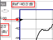
Scale annotation on the FieldFox screen Reference Line = red arrow Ref Level = -40 dB Ref Position = 1 Scale = 2 dB per division |
|
Trace Averaging helps to smooth a trace to reduce the effects of random noise on a measurement. The FieldFox computes each data point based on the average of the same data point over several consecutive sweeps.
Average Count determines the number of sweeps to average; the higher the average count, the greater the amount of noise reduction.
An average counter is shown in the left edge of the screen as Avg N. This shows the number of previous sweeps that have been averaged together to form the current trace. When the counter reaches the specified count, then a ‘running average’ of the last N sweeps is displayed. Average Count = 1 means there is NO averaging.
This setting can be changed at any time without affecting calibration accuracy.
| Averaging is often used to increase the dynamic range of a measurement. To achieve the highest dynamic range, select NA mode and reduce the IF Bandwidth setting. Learn more about dynamic range in “Increase Dynamic Range” on page 118. |
1.Press BW 2.
2.Then Average N where N is the current count setting.
3.Enter a value using the numeric keypad. Enter 1 for NO averaging.
4.Press Enter.
5.While Trace Averaging is in process, press Sweep 3 then Restart to restart the averaging at 1.
Trace smoothing averages a number of adjacent data points to smooth the peak-to-peak noise values on a displayed trace. The number of adjacent data points that are averaged is known as the smoothing aperture. Aperture is set by specifying a percentage of the X-axis span.
Trace smoothing does NOT significantly increase measurement time.
Smoothing can be used with any CAT format.
When enabled, Smo appears on the FieldFox screen.
How to set Smoothing
1.Press BW 2.
2.Then Smoothing ON OFF.
3.Then Sm. Aperture and enter a value between 0 and 25 (percent) using the numeric keypad.
4.Press Enter.
This setting determines whether the FieldFox sweeps continuously or only once each time the Single button is pressed. Use Single to conserve battery power or to allow you to save or analyze a specific measurement trace.
This setting can be changed at any time without affecting calibration accuracy.
How to set Single or Continuous
—Press Sweep 3.
—Then choose one of the following:
—Single Automatically sets Continuous OFF and causes FieldFox to make ONE sweep, then hold for the next Single key press. Hold is annotated in the upper left corner of the display when NOT sweeping, and changes to an arrow --> while the sweep occurs
—Continuous Makes continuous sweeps. This is the typical setting when battery power is not critical.
You can also use Run / Hold +/- to toggle between Single and Continuous.
Resolution (Number of Data Points)
Data points are individual measurements that are made and plotted across the X-axis to form a trace. Select more data points to increase measurement resolution. However, more data points require more time to complete an entire measurement sweep.
When the Resolution is changed after a calibration is performed, the calibration becomes interpolated. Learn more in “Interpolation *” on page 149.
1.Press Sweep 3 > Resolution.
2.Then choose one of the following:
101 | 201 | 401 | 601 | 801 | 1001 |1601 | 4001 | 10001.
Using SCPI, or measurement quick settings table, Resolution can be set to any number of points between 3 and 10001. See the Programming Guide at https://www.keysight.com/us/en/lib/resources/service-manuals/keysight-fieldfox-library-help-and-manuals-2153870.html.Learn more, “Quick Settings Table” on page 58.
The fastest possible sweep time is always used as the default setting. Use the Min Swp Time setting to slow the sweep time when measuring long lengths of cable.
Learn more in the FieldFox Supplemental Help at: https://rfmw.em.keysight.com/wireless/helpfiles/FieldFoxOnlineSupplementalHelp/Home.htm.
The actual sweep time is shown on the FieldFox screen. See “Take the FieldFox Tour” on page 44. To increase the sweep time, enter a value that is higher than the actual sweep time. The increase will not be exactly the amount that you enter, as the actual sweep time is the composite of many factors.
| Measurement speed specifications do NOT apply in Temperature Control Mode. Learn more in Chapter 1, “Overview.” |
—Press Sweep 3 > Min Swp Time.
—Enter a value using the numeric keypad.
—Press a multiplier key. Learn more in “Multiplier Abbreviations” on page 53.
Set the power level out of the FieldFox to High, Low, or manually set power level to a value between High and Low.
Generally, the high power setting is used when measuring passive, high-loss devices to place the signal farther from the noise floor. Increasing the power can also help reduce trace noise. However, for devices that are sensitive to high power levels such as amplifiers, use the Low power setting.
For best measurement accuracy, use the Manual power setting at –20 dBm. After calibration, the power level can be decreased for amplifiers, or increased for higher dynamic range.
Power Level settings in this mode will NOT change Power Level settings in other modes. To help prevent damage to your DUT, use caution when changing modes with your DUT connected to the FieldFox test ports. |
| For consistency with other FieldFox A/B models (backward compatibility), the default Output Power is set to –15 dBm. To avoid overload when using FieldFox C model, users should manually change the Output Power setting to –20 dBm. |
1.Press Meas Setup 4 > Power
2.Then Output Power
—High Sets output power to the maximum achievable power at all displayed frequencies. Output power is NOT FLAT across the displayed FieldFox frequency span. Use the High power setting, when better dynamic range and lower noise is desired. Please see Appendix B:, “Specifications/Data Sheet,” on page 979 for expected power levels.
—Low Sets output power to approximately –50dBm, FLAT across the displayed FieldFox frequency span.
—Man (Default setting) Sets the output power to –15 dBm, FLAT across the displayed FieldFox frequency span. If flattened power can NOT be achieved, a warning message and beep occurs. To achieve a flattened output power, reduce the power level or stop frequency.
—Then press Power Level
—Then enter a value using the numeric keypad, the arrows, or the rotary knob.
—Press Enter.
Use this setting when you suspect that other signals in the area are interfering with a measurement. Interference may look like a spike or lack of stability in the measurement trace. While monitoring a measurement at a specific frequency, toggle this setting between ON and OFF. If the measurement result decreases while ON, then there is an interfering signal in the area. Continue to make measurements with Interference Rejection ON. However, this will slow the measurement speed.
Once enabled, up to SIX sweeps may be required before the interfering signal is neutralized.
This setting can be changed at any time without affecting calibration accuracy.
How to set Interference Rejection
1.Press Meas Setup 4 > Interference Rejection [current setting].
2.Then choose from the following:
—Off No interference rejection and fastest possible sweep speed
—Minimum The lowest level of Interference rejection.
—Medium The medium level of Interference rejection.
—Maximum The highest level of Interference rejection.
This setting, especially useful for a Return Loss & DTF measurement, allows both measurements to have different frequency ranges.
With a Return Loss & DTF measurement present:
1.Press Meas Setup 4.
2.Select the DTF measurement (Tr2) using the arrows.
3.Then choose from the following:
—Coupled Freq ON - Both the Return Loss and DTF traces have the same frequency range settings.
—Coupled Freq OFF (default setting) - Both traces are allowed to have individual frequency range settings. When set to OFF:
—The Return Loss measurement frequency settings are made in the usual manner. Learn how at “Frequency Range” on page 59. When a new Start or Stop frequency is selected, Coupled Frequency is automatically set to OFF.
—The DTF measurement is made using the frequencies as determined by the DTF Frequency Mode setting. Learn more in “DTF Measurement Settings” on page 72.
Return loss can be thought of as the absolute value of the reflected power compared to the incident power.
When measuring an OPEN or SHORT, all incident power is reflected and approximately 0 dB return loss is displayed.
When measuring a LOAD, very little power is reflected and values of 40 dB to 60 dB are displayed.
The minus sign is usually ignored when conveying return loss. For example, a component is said to have 18 dB return loss, rather than –18 dB.
—Connect the jumper cable or any adapter used to connect the device under test (DUT).
—Select Preset then Preset Returns the FieldFox to known settings
—Select Mode then CAT/TDR (Cable and Antenna Test)
—Then Return Loss (Default measurement).
—Press Freq/Dist and enter Start and Stop frequency values of the measurement.
—Press Meas Setup 4 then Settings to make appropriate settings before calibrating.
—Disconnect the jumper cable or DUT and press Cal 5 then follow the calibration prompts.
—Reconnect the jumper cable or DUT.
—The return loss trace is displayed on the FieldFox screen.
1-Port Cable Loss Measurements
While all cables have inherent loss, weather and time will deteriorate cables and cause even more energy to be absorbed by the cable. This makes less power available to be transmitted.
A deteriorated cable is not usually apparent in a Distance to Fault measurement, where more obvious and dramatic problems are identified. A Cable Loss measurement is necessary to measure the accumulated losses throughout the length of the cable.
A 2-port Insertion Loss measurement is usually more accurate than a 1-port Cable Loss measurement. However, to perform a 2-port Insertion Loss measurement, both ends of the cable must be connected to the FieldFox.
| In high-loss conditions, a Cable Loss measurement becomes ‘noisy’ as the test signal becomes indistinguishable in the FieldFox noise floor. This can occur when measuring a very long cable and using relatively high measurement frequencies. To help with this condition, use High Power (page 63) and Averaging (page 60). |
How to make a 1-port Cable Loss Measurement
1.Press Preset then Preset.
2.Then More then Cable Loss (1-Port)
3.Connect the cable to be tested.
4.Press Freq/Dist and enter Start and Stop frequency values of the measurement.
5.Press Sweep 3 then Min Swp Time. Increase the Sweep Time until a stable trace is visible on the screen. The amount of time that is required increases with longer cable lengths. Learn more in the Supplemental Online Help at: https://rfmw.em.keysight.com/wireless/helpfiles/FieldFoxOnlineSupplementalHelp/Home.htm.
6.Remove the cable to be tested.
7.Press Cal 5, then Mechanical Cal.
8.Follow the prompts to perform calibration at the end of the jumper cable or adapter. Learn more about Calibration in “How to Perform a Calibration” on page 134
9.Connect the cable to be tested.
| Low-level standing waves (also known as ‘ripple’) which may be visible in reflection measurements, can hide the actual loss of the cable. Steps 10 through 13 can minimize the ripple. Perform the measurement with and without steps 10 through 13 and choose the method with the least amount of ripple. |
10. Connect a LOAD at the end of the cable to be tested. This limits the reflections to faults that are located in the cable under test.
11. Press Trace 6 then Math and Memory then Data->Mem to store the trace into Memory.
12. Remove the LOAD and leave the end of the cable to be tested open.
13. Press Data Math then Data – Mem. The ripple in the measurement is removed. These minor imperfections in the cable should not be considered in the Cable Loss measurement.
14. Use Averaging to remove random noise from high-loss measurements. Press BW 2 then Average.
The displayed trace shows the Cable Loss values in one direction through the cable. A Return Loss measurement would show the loss for both down the cable and back. Therefore, a Cable Loss measurement is the same as a Return Loss measurement divided by 2.
The average Cable Loss across the specified frequency range is shown on the screen below the graticules.
2-Port Insertion Loss Measurements
A 2-port Insertion Loss measurement is used to measure the loss through a DUT (device under test) – or cable – over a specified frequency range. The FieldFox signal source is transmitted out the RF OUT connector, through the DUT, and into the RF IN connector. Both ends of the DUT must be connected to the FieldFox, either directly or indirectly using the cable used in the normalization cal.
‘Insertion’ loss simply means loss through a device, usually expressed in dB. It is exactly the same measurement as “S21 Transmission” in NA Mode. Exception: In CAT mode, if the TDR data are saved in S1P format, the values represent the real part of the complex transform; the imaginary part is set to zero. To obtain complex data, either as real/imaginary or magnitude/phase pairs, use NA mode.
2-port Insertion Loss measurements are generally more accurate than 1-port Cable Loss measurements.
How to make a 2-port Insertion Loss Measurement
—Press Mode then CAT.
—Then More then Insertion Loss (2-Port).
—Press Freq/Dist and enter Start and Stop frequency values of the measurement.
—Press Sweep 3, then select a Resolution setting.
—Press Cal 5, then perform a calibration. Learn more on “How to Perform a Calibration” on page 134.
—Connect the DUT and view the insertion loss measurement results.
When measuring very long lengths of cable, it may be necessary to increase the sweep time. Learn how on page 62. Learn how in the Supplemental Online Help at: https://rfmw.em.keysight.com/wireless/helpfiles/FieldFoxOnlineSupplementalHelp/Home.htm.