Note: This feature was previously known as Multi-channel Eye Diagram
Add advanced effects to simulated Transmitter and Crosstalk data sources, and add equalization to the Receiver for eye diagram simulation.
In this topic:
AMI Settings for TX, XT TX, and RX modules
Transmit (TX) and Crosstalk (XT TX) Source Settings dialog box
Bit Pattern tab - Specify bit pattern settings for data sources.
Jitter tab - Add jitter to the data sources.
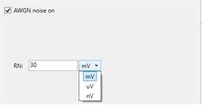
AWGN tab -Add source noise.
Pre-emphasis tab - Add source equalization.
Receiver (RX) Settings dialog box - Add linear equalization.
See Pre/De-emphasis example (separate topic)
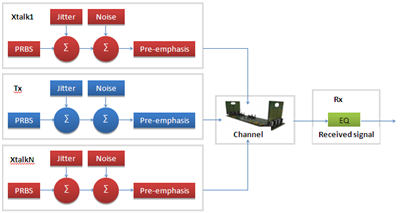
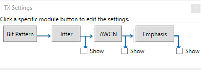
The following flow diagram shows how simulated Jitter, Noise, and Emphasis can be added to transmitter to stimulate your DUT.
Add and configure ONE Transmit (TX) component to a channel.
Add and configure ONE Receiver (RX) component to a channel.
Add and configure Cross-Talk (XT TX) components to the transmitter and/or receiver.
Click Draw Eye to simulate how the channel reacts to these effects.
The simulation effects are computed using a run-time version of MATLAB® which is installed with PLTS.
Note: With a Multi-channel Simulation selected, you can view the enhanced Bit Pattern Waveforms. Learn how.
Open a data set in either Differential or Single-ended Eye Diagram view.
Click Tools, then Multi-channel Simulation.
ConfigurationsFrom this dialog, Multi-channel configurations are created, modified, and saved to your PC for reuse at a later time. The multi-channel simulation configuration is dependent on a specific DUT configuration. When you select another data set with a different DUT configuration, this window will automatically update the multi-channel simulation configurations that match the current DUT configuration in the list. This allows you to use one configuration to simulate the eye diagrams of many data sets that have the same DUT configuration. Existing configurations Select the configuration to be used or modified. The configurations that appear are those that are resident in PLTS memory. Configuration1 is an empty configuration if none are present. Add a new configuration with name... Type a name in the field, then click Add. The configuration is added to the Existing configurations and selected. Delete Select a configuration, then click Delete to remove the configuration from PLTS memory. Rename Select a configuration, type a new name in Rename selected configuration, then click Rename. Save After modifying one or more configurations, click Save to store the selected configurations on your PC. When more than one configuration exists, the Select configurations to save dialog is launched. Select one or more configurations to save in the file. Load Recall a configuration from your PC hard drive.
|
Right-click on an AMI slot component to Edit or Delete the properties of that component. This dialog is used to load a vendor-supplied model for the following components:
The yellow areas represent the vendor-supplied AMI models See AlsoLearn more about the IBIS-AMI standard.
Browse Click to navigate to the (*.ibis) file to be loaded. The associated (*.ami) file and supporting files are loaded automatically. View Click to see a text-file representation of the IBIS and AMI files. Component - Shows the root parameter name in the AMI file. Corner settings - Used to simulate the corner cases. For AMI parameters defined as Corner, PLTS will pick one of the three supplied values (<typ value>, <slow value>, <fast value>) in the parameter definition file for any given model instance. This selection is governed by the same internal corner variable that controls the selection of the "Typ", "Min", "Max" model data.
AMI Parameters
RX AMI Settings
Show RX input waveform - When checked, an additional eye diagram at the input of the RX is shown after simulation. The remainder of these settings are identical to the TX AMI settings. |
TX (source) and XT TX (crosstalk source) Settings dialog box help |
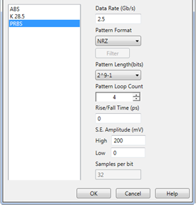
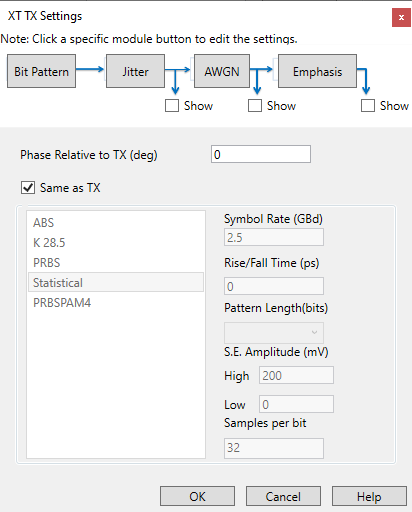
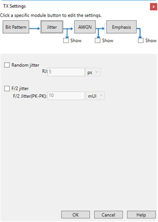
Click a box to show the dialog settings: Bit Pattern Jitter AWGN Emphasis Show Check individual boxes to create additional eye diagram plots with ONLY the selected effects at each node. These eye diagrams are in addition to a plot of the simulated transmitted signal. Bit Pattern tabThe available settings for this tab vary between TX and XT TX dialogs. The image below shows the Bit Pattern dialog for TX Settings. The image below shows the Bit Pattern dialog for XT TX Settings.
Phase relative to TX (deg) (XT TX dialog only) Enter a phase to offset from the transmitted port. This allows the XT TX setting to be more visible in the resulting Eye Diagram. Same as TX (XT TX dialog only)
Symbol Rate (GBd)/Select Enter a baud symbol rate in the text box or click on the Select button to select a baud symbol rate from the drop down menu. Pattern Format (TX dialog only) Select from the following:
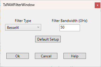
Filter This button is active ONLY when PAMn is the selected Pattern Format. It opens the TxPAMFilterWindow dialog shown below.
Filter Type Select between the following filter types:
Filter Bandwidth Bandwidth of the selected filter. Click Default Setup to reset the setup to its default setting. Pattern Length (bits) Select the desired pattern length from the drop down menu. Pattern Loop Count (TX dialog only) Set the number of times to loop through the pattern. Rise/Fall Time (ps) (TX dialog only) Set the rise and fall times (in picoseconds) of the transitions. S.E. Amplitude (mV) Eye diagram Y-axis scaling in millivolts. Negative voltages are allowed for differential eye diagrams; these scale values are doubled.
Samples per bit Set the number of samples for each bit. Jitter tab with NRZ Pattern FormatJitter is typically divided into deterministic and random jitter.
Learn more in the MATLAB documentation.
Same as TX (Appears ONLY on the XT dialog)
Random Jitter Check to enable random jitter.Random Std (ps) - Standard deviation of the random jitter in picoseconds. Used only when enabled. Periodic Jitter Check to enable periodic jitter.Add and Remove Several periodic jitter components with varying properties can be added. Click Add, then change the subsequent settings. Periodic amplitude (ps) - Amplitude of each sinusoidal component of the periodic jitter in picoseconds. Periodic frequency (Hz) - Frequency of each sinusoidal component of the periodic jitter in Hz. The default is 1 kHz. Periodic phase - Phase of each sinusoidal component of the periodic jitter. Dirac Jitter (ISI) Check to enable Dirac jitter.Add and Remove Several Dirac jitter components with varying properties can be added. Click Add, then change the subsequent settings. Dirac delta (ps) - Time delay of each Dirac component in seconds. Dirac probability - Probability of each Dirac component. Sum must be one. Jitter tab with PAM4 Pattern FormatThe following selections are displayed when PAM4 is selected as the Pattern Format in the Bit Pattern tab.
Same as TX (Appears ONLY on the XT dialog)
Random jitter Check to enable random jitter.RJ (ps) - Standard deviation of the random jitter in picoseconds. Used only when enabled. F/2 jitter Check to enable F/2 jitter.F/2 Jitter (PK-PK) - Every second bit, whether it is a zero or a one, is longer or shorter by the value entered in the F/2 Jitter (PK-PK) field. For example, 0.05 UI will make every second bit 5% (5% of the unit interval based on the data rate) longer or shorter. AWGN tab with NRZ Pattern FormatWhite Gaussian noise is injected from the data source. Learn more in the MATLAB documentation.
Same as TX (Appears ONLY on the XT dialog)
Symbol SNR (dB) Set the symbol signal-to-noise ratio in dB. AWGN tab with PAM4 Pattern FormatWhen the Pattern Format is PAM4, the random noise level can be set in mV, uV, or nV.
Emphasis tabConcepts: In serial data transmission, pre-emphasis/de-emphasis is often used to compensate for losses over the channel which are larger at higher frequencies. The high frequency content is emphasized compared to the low frequency content which is de-emphasized. This is a form of transmitter equalization.
The dB value can control how much the signal is enhanced or declined. A 2-tap FIR filter is automatically applied with the specified dB values. Pre-emphasis is used to enhance the first bit level after a transition.
De-emphasis is used to decline all the bit levels except the first bit after a transition.
Same as TX (Appears ONLY on the XT TX dialog)
Choose emphasis method: None - Emphasis is disabled. Specify Pre-emphasis Enter a value in dB. A 2-tap FIR filter is automatically applied. Specify De-emphasis Enter a value in dB. A 2-tap FIR filter is automatically applied. Specify FIR (filter) taps The filter function is implemented in MATLAB as a direct form II transposed structure. Learn more in the MATLAB documentation. Specify M-script file Add pre/de-emphasis with a custom MATLAB script file. Learn more in the MATLAB documentation. |
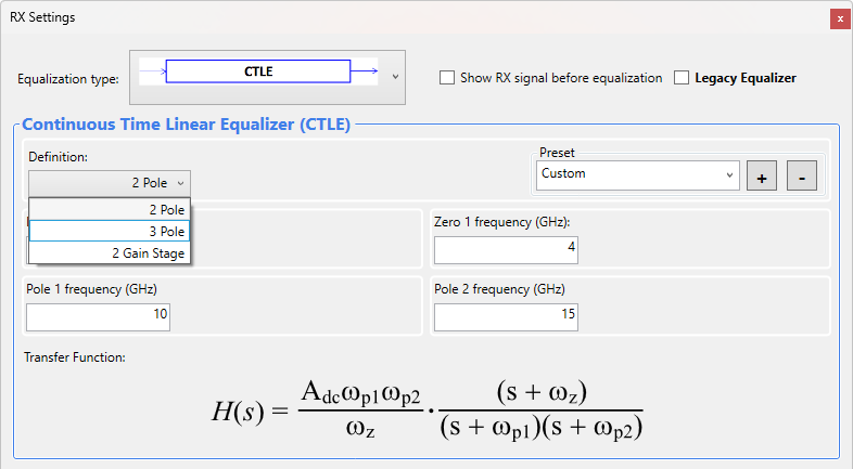
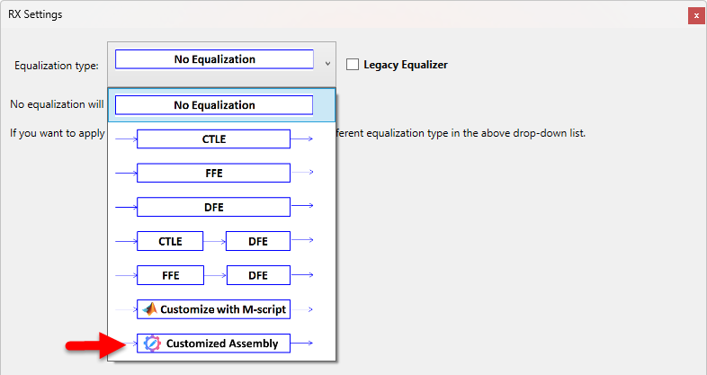
Channel equalization is a simple way of mitigating the detrimental effects caused by a frequency-selective and dispersive communication link between transmitter and receiver. Learn more about Equalization in this Keysight App Note: http://literature.cdn.Keysight.com/litweb/pdf/5990-3585EN.pdf Choose from:
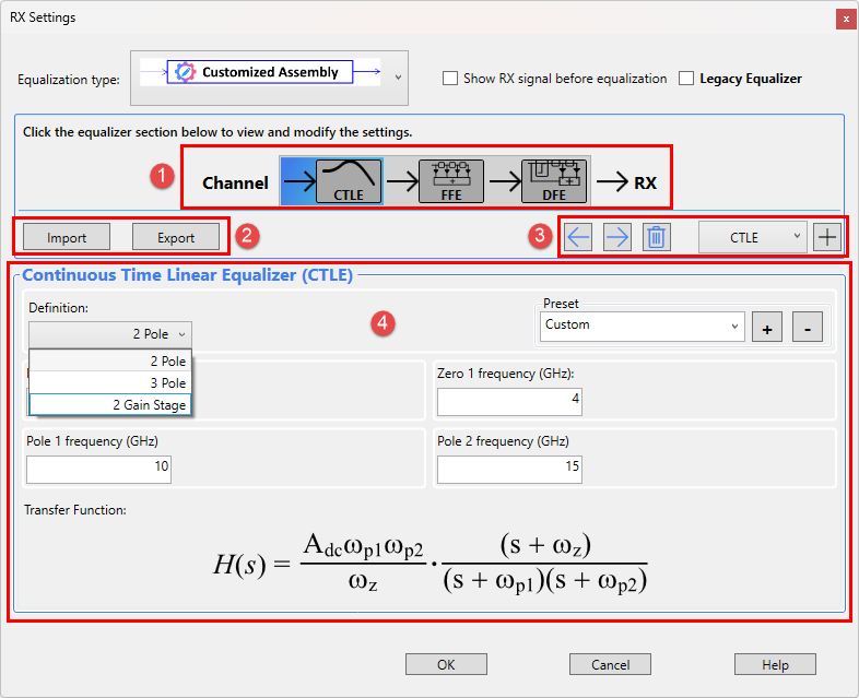
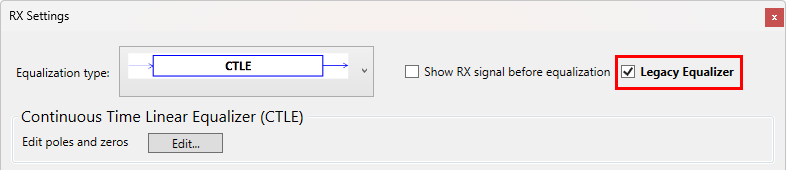
CTLE (Continuous-time Linear Equalizer)This is the new CTLE equalizer interface for PTLS 2026. You can still use the Legacy Equalizer by clicking the checkbox.
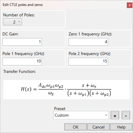
Legacy EqualizerSpecify the equalizer using poles and zeros.
Show RX signal before equalization
Edit poles and zeros. Click Edit to show the following dialog:
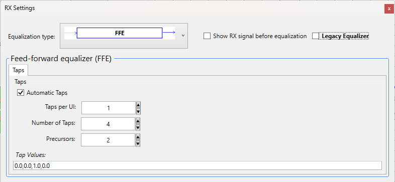
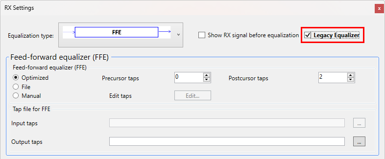
FFE (Feed-forward equalizer)This is the new FFE equalizer interface for PTLS 2026. You can still use the Legacy Equalizer by clicking the checkbox.
Legacy EqualizerLearn more about FFE Equalization in this Keysight App Note: http://literature.cdn.Keysight.com/litweb/pdf/5990-3585EN.pdf
Show RX signal before equalization
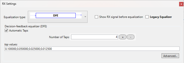
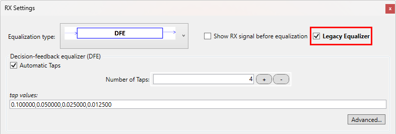
Feed-forward equalizer (FFE)Optimized The Pre/Post cursor taps are selected automatically. Specify the number of taps that you need. File Tap file (for FFE or DFE) - To load a *.tap file, click Browse, then navigate to *.tap files. Learn more about Tap Files Manual - Click edit to launch the Edit FFE Taps dialog box where you can create and edit filter taps. DFE (Decision-feedback Equalizer)This is the new DFE equalizer interface for PTLS 2026. You can still use the Legacy Equalizer by clicking the checkbox.
Legacy EqualizerLearn more about DFE Equalization in this Keysight App Note: http://literature.cdn.Keysight.com/litweb/pdf/5990-3585EN.pdf
Show RX signal before equalization
Automatic Taps - Check to use automatic tap values or uncheck to use manual entry tap values.
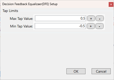
Advanced... - Opens the Decision Feedback Equalizer (DFE) Setup dialog to enter the maximum and minimum tap limit values. Enter the values directly into each text box or use the "+" and "-" keys to change the values.
Equalization CombinationsThe following two equalizations use combinations of the above CTLE, DFE, and FFE equalizations. The equalizations are processed sequentially. Either CTLE or FFE, then DFE. See the individual equalization types for help with each component. CTLE =>DFESee CTLE and DFE equalizations.
FFE=> DFESee FFE and DFE equalizations.
Customize with M-script
Provide a MATLAB script file that describes your custom equalization. Customized AssemblyThis is a new feature with PLTS 2026.
Using the Customized Assembly:By default, the equalizers are applied in this sequence: CTLE > FFE > DFE. Refer to the descriptions and the image below. Select the equalizer section block (area 1) to view and modify the settings (area 4). Export (area 2) the current assembly sequence to an *.xml file. Import (area 2) the equalizer sequence from a file (*.xml). Sequence Edit (area 3):.
|
Appears when Edit Taps (Manual) is clicked on the RX FFE Settings dialog.
|
Appears when Edit Taps (Manual) is clicked on the RX DFE Settings dialog.
|
Use Input Tap files to specify the tap values to used in FFE or DFE equalization.
When Optimized is selected, the Tap values are selected automatically by PLTS. When a path and filename is specified for Output taps, the tap values that were automatically selected are output to the file. This file can then be specified for Input taps in subsequent equalization simulations.
The following file was Output from a FFE->DFE equalization. Two taps each are specified for Precursor, Postcursor, and DFE Taps.
This same format is used for Input files.
For FFE-only, do NOT specify DFETap values.
For DFE-only, do NOT specify Pre/PostCursor values.
Click File, then Open then navigate to [DEMO] E8362B BTL 10MHz-20GHz.dut.
On Analysis Type, select Eye Diagram (single ended).
Click Tools, then Multi-channel Simulation
Drag a Tx component to port 1.
Right click the Tx channel, then click Edit, then make the following Pattern settings: .5 Gbps, 80 ps rise/fall time, PRBS 2^9 -1, 0~200 signal amplitude.
Turn OFF Tx jitter, pre-emphasis, and noise of the Tx component.
Drag a RX component to port 2.
Turn OFF RX equalization. This allows us to see ONLY the Tx signal transmitted through the backplane channel. Later we can see only the effect of crosstalk by comparison.
Click Draw Eye
Right click the TX component of port 1, then click Edit.
Change to port 3 so that we can simulate only the eye diagram of T23 crosstalk.
Leaving the other settings unchanged.
Click Draw Eye
Move the TX back to port 1.
Add a XT TX component to port 3. Note that the small “hill” in the crosstalk picture of step 2 is the rising and falling edge of the crosstalk eye. If the transmission channel delay is very close to the XT TX channel delay and there’s no user-specified XT TX delay, the XT TX eye will synchronize with the transmission eye and we can’t clearly see the crosstalk effect.
To clearly see the effect of the crosstalk, add 180 degrees (half bit period) phase shift to the XT TX compared to TX.
Click Draw Eye
The crosstalk “hill” should be in the center area of the transmission channel eye diagram.
 Move selected equalizer forward
 Move selected equalizer backward
 Delete selected equalizer from sequence
 Select from CTLE, FFE, and DFE to add to sequence
 Add the equalizer to the sequence