De-embedding Operators

The 2 Port and 4 Port ee-embedding operators provide the most precision for removing or inserting test-setup elements. Click on these operators to create a network that describes the full system of transmitter, receiver, and channel blocks. For each block, both measurement and simulation electrical circuits are defined:

• The measurement circuit models the actual physical electrical circuit that produced the measured waveform.
• The simulation circuit models a hypothetical electrical circuit that exhibits the characteristics that you want to measure.

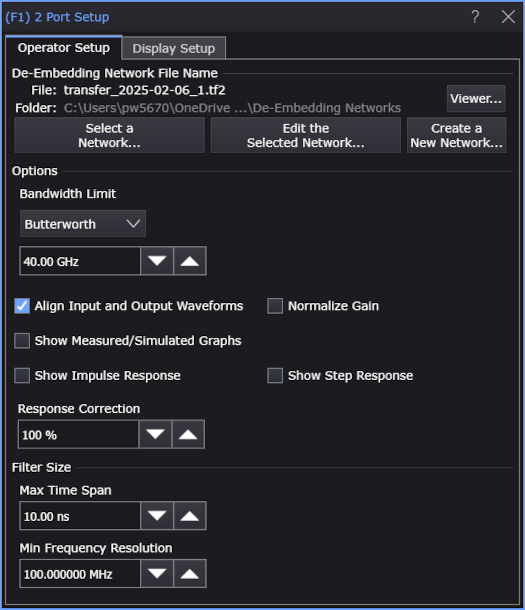
The first step when setting up a De-embedding simulation function is to specify the network that is applied to the input waveforms. You can:

• Select a Network... — If you have already have a transfer function file generated for the measurement and simulation circuits you want to apply, click this button to select and load the network file.
• Edit the Selected Network... — Once a network is selected (or created), click this button to change the network's configuration.

• Create a New Network...— Lets you define the de-embedding network (that is, measurement and simulation circuit models) from which transfer functions are generated and saved in files. See Setting Up a Network.

  In your definitions, you can enable the most complete waveform rendering by including the reflective S-parameter elements in the mathematical calculation of the correction transfer function file which is used to transfer data from the measurement to the simulated (displayed) measurement.

Click Viewer... to open the S-Parameter/Transfer Function Viewer where you can chart S-parameter and transfer function responses.

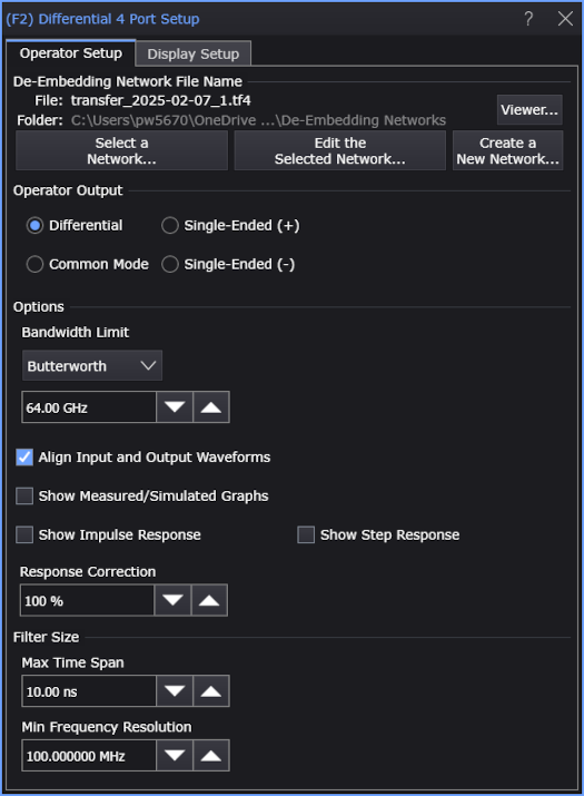
Operator Output

Use the Operator Output controls to specify the type of output waveform.

With a Differential 4 Port function (that has two inputs for a four-port transfer function network file):

• Differential — Outputs the differential sum from a 4-port transfer function.
• Common Mode — Outputs the common-mode sum from a 4-port transfer function.
• Single-Ended (+) — Outputs the single-ended plus side from a 4-port transfer function.
• Single-Ended (-) — Outputs the single-ended minus side from a 4-port transfer function.

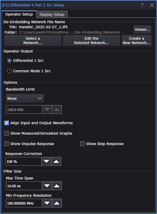
With a Differential 4 Port 1 Src function (that has one input for a four-port transfer function network file) where the differential or common-mode signal is created prior to de-embedding:

• Differential 1 Src — Extracts the differential path from a 4-port transfer function.
• Common Mode 1 Src — Extracts the common-mode path from a 4-port transfer function.

Options

Use the Bandwidth Limit option to minimize the effects caused by noise. See Bandwidth Limit.

Clear the Align Input and Output Waveforms field to view the delay introduced by your device. By default, this field is normally selected and the input and output waveforms are aligned.

Select Normalize Gain to remove any DC gain of the transfer function. This can be used when modeling probes.

The Show Measured/Simulated Graphs option displays a Freq-Mag window that contains:

• The measured signal's frequency response.
• The simulated signal's frequency response (the signal after De-embedding transforms the measured signal).
• The correction transfer function's frequency response. With 0% (no) Response Correction, this frequency response plot will be flat.

These plots can help you verify the de-embedding definition or sometimes see errors in the transformation or problems with the transfer function. These plots can also help you determine what value to use for the bandwidth limit based on where your signal's frequency response is mostly just noise. See Measured/Simulated Graphs Example.

The Show Impulse Response and Show Step Response options automatically load the selected network file into the S-Parameter/Transfer Function Viewer and add impulse response and step response charts if the parameters can be determined; otherwise, you can add these charts by selecting the proper parameters.

The Response Correction field linearly scales the amount of correction applied to the non-DC frequency components of the measured signal. This lets you trade off the amount of correction to apply through the transformation function versus the increase in noise it may create at higher frequencies. In other words, you can fine-tune the amount of high-frequency noise versus the sharpness of the step response edge.

If you are making averaged mode measurements or applying a transfer function that does not magnify the noise, use the full correction by setting the Response Correction field to 100%. However, if you are working with eye diagrams or making jitter measurements and the transfer function is magnifying the noise, you may want to limit the correction by selecting a lower percentage.

Once you have your transformed signal displayed on screen, you can adjust the Response Correction value in the dialog box to see its effect on the signal.

It is also useful to display the frequency response plots and step response plot while you adjust the Response Correction field to see its effect on these plots. For instance, you can see how the frequency response of the transformation filter changes as you change the percentage. See S-Parameter/Transfer Function Viewer.

Filter Size

The Filter Size area has two controls: Max Time Span and Min Frequency Resolution. These two controls are reciprocals of each other and tied together, so as you set one to a lower value, the other one raises to a higher value and vice versa. The correction transfer function is applied by means of a FIR digital filter. The size of this filter determines the time span of the transformation it can apply. However, there is a trade-off. Using a longer filter corrects longer time constants, but it can take longer to calculate. By default, Infiniium tries to choose a filter size that preserves the coarsest frequency resolution used by all of the model blocks. However, you can limit the filter size by reducing the Max Time Span value.

A quick summary of the two controls is:

• Increasing the Max Time Span control increases the maximum time span of the correction transfer function's impulse response. Increasing this control enables Infiniium to apply transformations that have slower time constants. You can use either the Step Response or Impulse Response plot to see if the time span is long enough to model your device adequately.
• Increasing the Min Frequency Resolution control makes the frequency resolution less fine and automatically decreases the Max Time Span control (which corresponds to a higher update rate). Therefore, you would do this if you wanted a higher update rate with the trade-off of a shorter transfer function impulse response. Generally, you want to set the Max Time Span using the Step Response or Impulse Response plot and then this Min Frequency Resolution is set automatically.

Display Setup

Each operator's setup includes a Setup section that has the selections that are shown in the following generic setup dialog box. Use these settings to control the display of the operator's output waveform, including turning the display on or off. Use the Name field to display an identifying name to the waveform which can be helpful for screen captures or when multiple waveforms are displayed. The settings also include the output waveform's color, scaling, and signal type. The scaling Automatic selection allows the output waveform to track changes to the scaling of the input waveform. This is the setting that you would normally want to use.

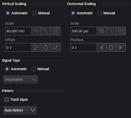
The signal Pattern can be used for BER (Bit Error Ratio), SNDR (Signal to Noise and Distortion Ratio), and other measurements. You can specify the math function has the same pattern as the input waveform (Track Input), Auto Detect the pattern, choose a Known Pattern from a list, or specify your own pattern using a Pattern File.