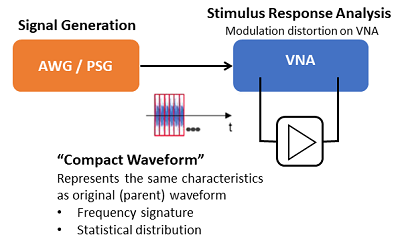
The Modulation Distortion application characterizes the nonlinear distortion of RF microwave amplifiers and converters under a modulated signal.
In this topic:
Unprecedented dynamic range through coherent averaging (repetitive waveforms are used)
Corrects for port match and establishes calibration reference plane (VNA vector error correction is applied)
No need to demodulate the response signal
Accurate measurement of modulated signal with VNA receivers
Analysis of nonlinear behavior of the device under modulated signal stimulus
Measure input and output signals coherently
Delivers figure of merits of the device commonly used in the industry (ACP, EVM, NPR)
M98xxA-090 Spectrum analysis hardware
M983xA-270 with option 190 provides internal up-convertor for modulation measurement. It works closely with M983xA MOD application and SA multitone measurement.
Note: In multi-module configuration, the MOD is supported only when DUT Input/Output is connected to the same product family (M980xA or M983xA). Ex: Supported: DUT Input and Output are connected to M980xA. Not Supported: DUT Input: M980xA, DUT Output: M983xA
Note:[M983xA-270] The signal source over 6 GHz frequency is not required as the M983xA has an up-converter capability.
Note: When setting up an M9383A, M9383B, or M9384B source in the External Device Configuration dialog, select MXG_Vector as the driver (they are code compatible).
N5182B MXG X-Series RF Vector Signal Generator
N5192A and N5194A UXG Vector Adapter
M9410A, M9411A, M9415A and M9416A VXT
Note: [M983xA] The cable between M941xA RF Out and M983xA BB in is available as M9830-61610.
M941xA VXT with M9471A frequency extension module.
This up-converter intends to use with the MOD and SA multitone applications. General Tx up-converter using for demodulation analysis is not supported..
When up-convertor is enabled, internal CW source is disabled in the SA Source tab. This is because it’s used as a LO supply.
Manual IF and LO setting is not supported in the MOD / SA. They are selected fully automatically.
Other applications cannot control the up converter automatically. However, users can manually setup the up-converter using the Path Configuration.
On M9837A-271, the maximum modulation bandwidth is limited up to 550 MHz at the center frequency from 31.8 GHz to 37 GHz. The limit for the other center frequency is the same (2 GHz).
A Vector Signal Generator is used to generate a repetitive signal with a given CCDF (Complementary-Cumulative-Distribution-Function) and PSD (Power Spectral Density).
See the detailed hardware setup at Physical_Setup_for_M983xA-270 or Physical_Setup_M980xA.
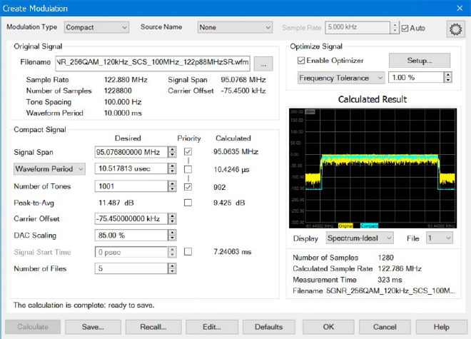
The modulation distortion application uses a short waveform period to perform an accurate measurement within a relatively short time frame. This process is known as compacting the waveform.
For example, use this process if you want to determine the response of the DUT using a waveform under a specific modulation scheme. The VNA firmware helps to create a slice of the parent waveform. The waveform inherits the frequency signature and statistical characteristics. The sliced waveform is called the compact test signal.
The parent waveform is created using the Keysight Signal Studio Software and is a .wfm file. (The parent waveform is also referred to as the original waveform.) In addition, you can use a .csv file format that has a timestamp, I, and Q that uses a comma to separate the values.
Note: Encrypted .wfm files created using the N5182B MXG RF Vector Signal Generator are not supported.
The following parent waveform is a 5G NR 100 MHz bandwidth signal:
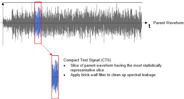
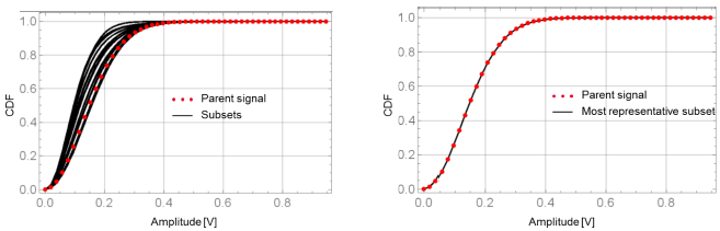
The PNA-X firmware uses a unique algorithm to determine the most statistically representative slice from the parent signal. The results are from the parameters selected in the Create Modulation dialog. The firmware then applies a brick wall filter to remove spectral leakage when the compact test signal plays.
The following shows the CDF of a parent signal and subset slice:
Depending on the parameters selected in the Create Modulation dialog, the compact test signal displays different characteristics, which can affect the measurement result.
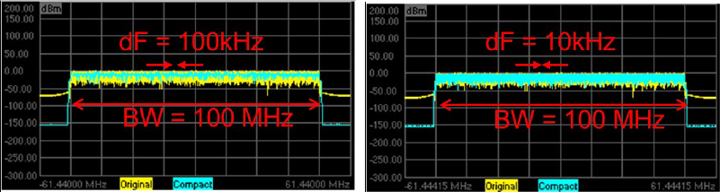
For example, if you are using a 5G NR 100 MHz bandwidth waveform as a parent waveform to create a compact test signal, the plots below illustrate two different compact test signal characteristics when using different parameters for the same parent waveform.
The yellow trace indicates the parent waveform, and the blue trace shows the compact test signal. The plots on the left display a compact test signal consisting of 1,001 tones with a 100 kHz tone spacing. The plots on the right display a compact test signal consisting of 10,001 tones with a 10 kHz tone spacing.
The following plots represent the spectrum of the waveform. The results show what the waveform looks like in the frequency domain by applying the Fast Fourier Transform (FFT) to each waveform. The frequency signature of signals in both the left and right plots have the same bandwidth as the original signal. The original signal has a higher out-of-band spectrum. The compact test signal has a low out-of-band spectrum that uses the brick wall filter for cleaning the signal.
|
CTS #1: 1,001 Tones |
CTS #2: 10,001 Tones |
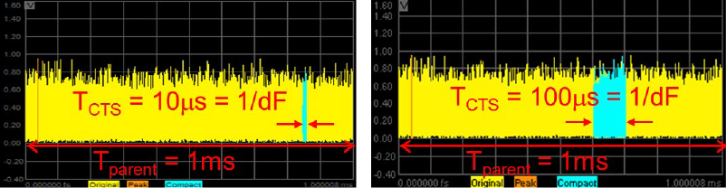
The following plots represent the position of a compact test signal within the parent signal in the time domain. The numbers shown represent the waveform length (reciprocal of the tone spacing). The left compact test signal has a waveform length of 10 us; the waveform length of the right compact test signal is 100 us. A finer tone spacing waveform results in an extended period of the compact test signal waveform.
|
CTS #1: 1,001 Tones |
CTS #2: 10,001 Tones |
The following plots represent the complementary cumulative distribution function (CCDF) curve of the parent signal, compact test signal, as well as Gaussian distribution (pink trace). The CCDF of this specific parent waveform is in alignment with the Gaussian distribution. The CCDF of a compact test signal that consists of 10,001 tones aligns with the parent waveform across the entire probability. The CCDF of a compact test signal that includes 1,001 tones aligns with the parent waveform, but only until it is approximately a 0.1% probability.
|
CTS #1: 1,001 Tones |
CTS #2: 10,001 Tones |
The following is a simplified block diagram of a modulation distortion setup showing the VNA receivers and VSG.
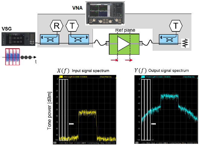
The VSG replays the compact test signal without any interruptions. Three VNA receivers capture the spectrum at the reference plane at the input and output of the DUT. The instantaneous bandwidth of the VNA ADC (Analog-to-Digital Converter) is at 30 MHz. When the modulation distortion application measures the spectrum of the signal with a bandwidth wider than 30 MHz, it moves the local frequency of the VNA to measure the spectrum for each instantaneous bandwidth. It then combines the captured partial spectrum to obtain a complete spectrum response.
When the modulation distortion application measures the spectrum for each section, it uses multiple receivers coherently and applies linear calibration terms. The modulation distortion application offers a measuring technique where the VNA completes accurate vector corrected measurements at the reference plane.
The block diagram above shows how the VNA measures the input signal and the output signal spectrum:
Signal generator generates a repetitive compact test signal.
VNA receiver measures the input signal spectrum and output signal spectrum in the frequency domain.
Output signal spectrum has spectral regrowth created by the nonlinear response of the DUT.
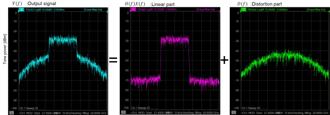
The DUT is stimulated with a low-level signal to measure its linear parameters and a high-level modulated signal to measure its distortion characteristics. The modulation distortion application processes the data and compares the input spectrum X(f) and the output spectrum Y(f) using a process known as spectral correlation. As a result, the modulation distortion application decomposes the output signal spectrum into two parts: H(f)*X(f) and D(f). H(f)*X(f) linearly correlates to the input while D(f) represents the distortion which does not correlate to the input.
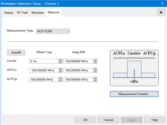
Computing ACPR is similar to the traditional signal generator and signal analyzer approach. The channel power of the in-band channel of interest and the channel power of the adjacent channel band is evaluated. The ratio between the BAND and AC is then computed.
For the EVM computation, the compact test signal plays continuously in the signal generator following the measurement of the input and output response of the DUT in the frequency domain. Spectrum correlation is then performed to compute the EVM.
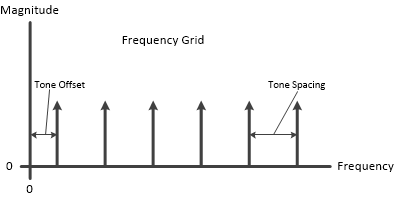
When viewed in the frequency domain, this signal is a mult-tone "grid" of frequencies. The data is measured on this multi-tone gird.
Poor EVM occurs when the random noise is the dominant factor of the EVM, where it likely happens at the left side of the bathtub curve. Improving the SNR of the measurement can improve the accuracy of the measurement.
The resolution bandwidth and the number of coherent averaging of the measurement determine the noise bandwidth. The default value of the noise bandwidth is 1 kHz. Noise bandwidth determines the signal-to-noise ratio (SNR) of the measurement system and measurement time.
As noise bandwidth decreases, modulation distortion increases the underlying coherent average. The result is a wider signal noise ratio and longer measurement time. The resolution bandwidth is set automatically with firmware from the compact test signal waveform length; it is a discrete number. It is the closest value to the one you entered.
The SNR of the VSG differs depending on multiple factors. A key factor is the number of tones of the compact test signal. As you increase the number of tones, the SNR of the VSG degrades. For example, compare a compact test signal with 1,000 tones and a compact test signal with 10,000 tones given the same channel power: -10dBm.
The tone power level of the compact test signal with 1,000 tones is -40 dBm, while the tone power of the compact test signal with 10,000 tones is -50 dBm. If the measurement has the same noise floor for each compact test signal, the compact test signal with 1,000 tones is 10 dB better than the compact test signal with 10,000 tones.
If there is a nonlinear response in the test receiver, it is unable to distinguish nonlinearity that comes either from the DUT or the receiver of the test system. The PNA-X test receiver needs to be in linear when measuring the signal. When it measures the subtle nonlinearity of a DUT, such as the EVM level of 1%, the recommendation is to keep the power level less than -5 dBm at the test port of the PNA-X. Use the receiver attenuator to adjust the power level if the test port power is higher than -5 dBm.
The linear error due to the test system can be corrected to have the desired compact test signal at the reference plane. You can do this by adjusting the channel power and linear flatness response using the modulated correction feature. Also, out-of-band spectral regrowth is suppressible by adjusting the ACPR.
It is critical to understand that nonlinear characteristics of the DUT under modulated signal condition is highly dependent on the stimulus signal. It is also important to create the compact test signal that can stimulate the DUT with the most representative statistical characteristics to the practical usage of the DUT.
The best practice is to align the complementary cumulative distribution function (CCDF) of the compact test signal with the parent waveform. However, the CCDF is not the same since the compact test signal is a slice of the parent waveform. The recommendation is to match the CCDF until it is 0.1% of probability. By choosing more than 3,000 tones gives you a good match of the CCDF — up to 0.1%.
Faster measurement time gives faster throughput to complete the evaluation. You can determine measurement time using these parameters:
signal analyzer span
noise bandwidth
compact test signal number of tones
Measurement time and measurement accuracy is generally a trade-off. It is essential to have the right balance of speed and accuracy to modify the parameter depending on the target measurement value.
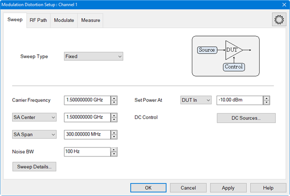
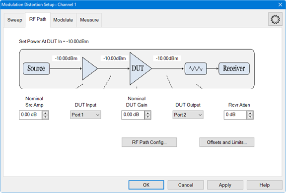
The GUI consists of setup dialogs accessed by clicking on their corresponding tabs. In this way, configurations can be set up quickly. See Configuring Distortion Measurements for information about these dialogs.
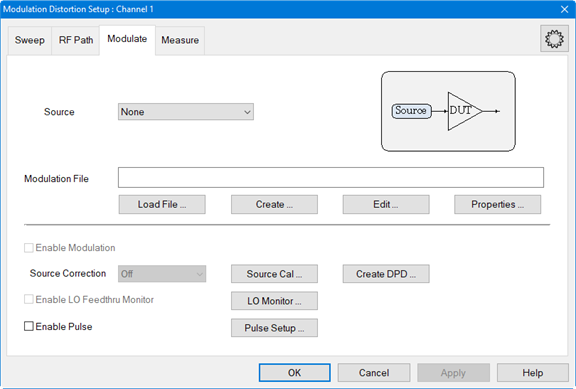
The Create... button in the Modulate tab accesses the Create Modulation dialog used to set up the compact test signal. See Creating Modulation Files for information about this dialog.