Spectrum Analyzer  

Configure SA settings

Using Hardkey/SoftTab/Softkey

Using a mouse

1. Press Freq > Main >  SA Setup....

1. Click Stimulus

2. Select SA Setup...

SA Setup Dialog tab help

For M983xA,

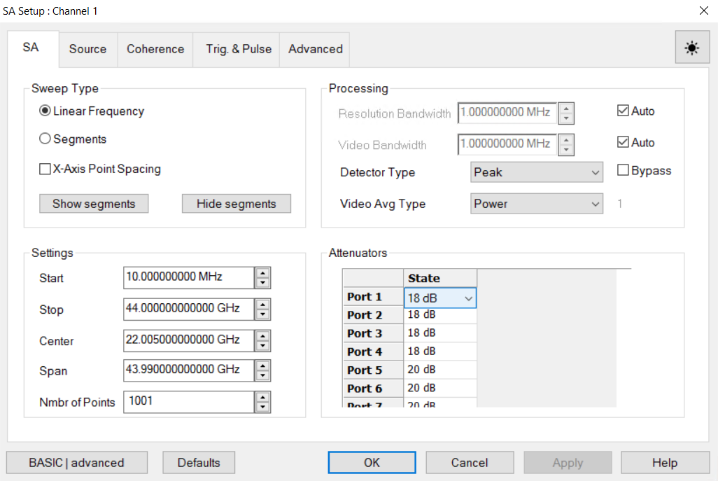
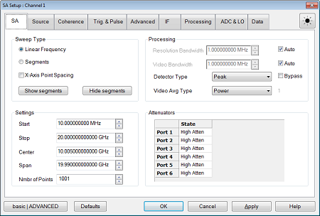
Sweep Type - Sets the spectrum analysis sweep type. See Type (Sweep).

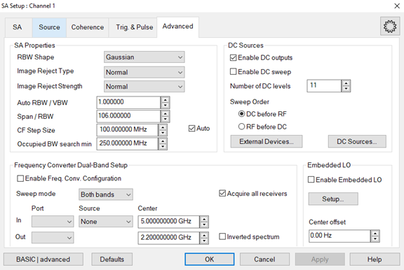
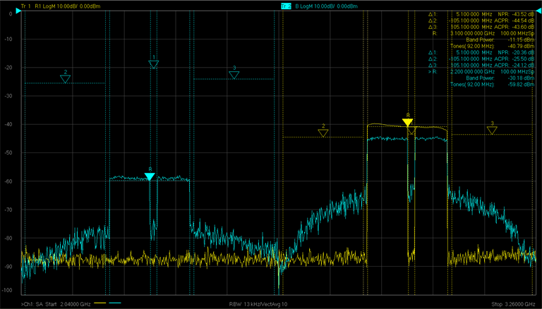
X-Axis Point Spacing - Enables or disables the separate segment sweeps in a Dual-Band Configuration for frequency conversion measurements. The span increases to display input and output signals.

Show segments - Displays the segment table at the bottom of the display. Number of points for each segment cannot be specified.

Hide segments - Hides the segment table.

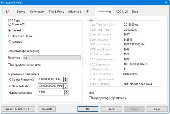
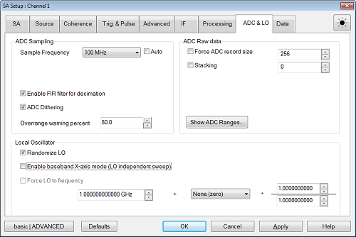
Processing

Resolution Bandwidth - Provides the ability to resolve, or see closely spaced signals. The narrower (lower) the Resolution Bandwidth, the better the spectrum analyzer can resolve signals. In addition, as the Resolution Bandwidth is narrowed, less noise is measured by the spectrum analyzer ADC and the noise floor on the display lowers as a result. This allows low level signals to be seen and measured. However, as the Resolution Bandwidth is narrowed, the sweep speed becomes slower.

Auto - Check to couple Resolution Bandwidth to the frequency span in a ratio based on the Span/RBW setting. As the frequency span is narrowed, the Resolution Bandwidth is also narrowed providing increased ability to resolve signals. Clear to uncouple the settings.

Video Bandwidth - Sets the video averaging factor. The averaging operation is applied after the DFT (Discrete Fourier Transform) and before the image rejection. The trace data is smoothed with the method selected by the Video Averaging Type. More smoothing occurs as the Video BW is set lower. However, as the Video BW is narrowed, the sweep speed becomes slower. The Video Bandwidth can be set from 3 Hz to 3 MHz when Auto is deselected. The VBW feature is emulated with averaging (see below the Averaging count). The averaging factor is computed with this equation: Round(0.8 + 0.38 * RBW / VBW).

Auto - Check to couple the Resolution Bandwidth to the Video Bandwidth in a ratio based on the RBW/VBW setting. Clear to uncouple the settings.

Detector Type - A "detector" is an algorithm used to map DFT bins into display buckets. There are typically several DFT bins in a single display bucket, and the detector determines how to translate the multiple DFT values into a single display value.

Peak - Displays the maximum value of all the measurements in each bucket. This setting ensures that no signal is missed. However, it is not a good representation of the random noise in each bucket.

Average - Displays the Root Mean Squared (RMS) average power of all the measurements in each bucket.  This is the preferred method when making power measurements.

Sample - Displays the center measurement of all the measurements in each bucket.  This setting gives a good representation of the random noise in each bucket. However, it does not ensure that all signals are represented.

Normal - Provides a better visual display of random noise than Positive peak and avoids the missed-signal problem of the Sample Mode. Should the signal both rise and fall within the bucket interval, then the algorithm classifies the signal as noise. An odd-numbered data point displays the maximum value encountered during its bucket. An even-numbered data point displays the minimum value encountered during its bucket. If the signal is NOT classified as noise (does NOT rise and fall) then Normal is equivalent to Positive Peak.

NegPeak- Displays the minimum value of all the measurements in each bucket.

Peak Sample - Attempts to determine if the display bucket contains an actual signal, or just noise. If a signal is present, the Peak detector is used, otherwise Sample is applied.

Peak Average - Attempts to determine if the display bucket contains an actual signal, or just noise. If a signal is present, the Peak detector is used, otherwise Average is applied.

Fast Peak - Keeps the x-axis grid untouched and indicates the value of the largest DFT bin from the bucket behind each display point.

Bypass - Check to bypass the Detector Type to view all display points from the DFT. This is only available if the total number of DFT points can be handled by the display.

Video Averaging Type - Determines how to compute the video average. When Auto is selected, the optimum type of averaging for the current instrument measurement settings is selected. It averages the magnitude of the DFT bins. Averaging only applies if the video bandwidth is less than the resolution bandwidth.

Voltage - Selects averaging of the detected signal's magnitude and returns the result.

Power - Selects averaging of the detected signal's squared magnitude and returns the square root of the result.

Log - Selects averaging of the detected signal's natural logarithm of the magnitude and returns the exponentiated value of the result.

Voltage Max - Returns the maximum voltage (signal magnitude) measured during the averaging period.

Voltage Min - Returns the minimum voltage (signal magnitude) measured during the averaging period.

Averaging Count - Reads the number of Video bandwidth sweeps that are averaged together. This readout is displayed to the right of the Averaging Type selection (the small "1" shown in the dialog above). It can be read with the remote interface using the SENS:SA:BAND:VID:AVER:COUNt? command.

Settings

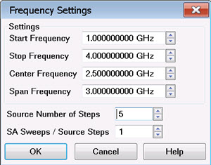
Sets the SA (receiver) frequency range when running Linear Frequency sweep type. Use either of the following pairs of settings to determine the frequency range.

Start /Stop - Specifies the beginning and end frequency of the swept receiver range. Start is the beginning of the X-axis and Stop is the end of the X-axis. When the Start and Stop frequencies are entered, then the X-axis annotation on the screen shows the Start and Stop frequencies.

Center /Span - Specifies the value at the center and frequency range. The Center frequency is at the exact center of the X-axis. The Frequency Span places half of the frequency range on either side of center. When the Center and Frequency Span values are entered, then the X-axis annotation on the screen shows the Center and Span frequencies.

Number of Points - Selects the number of trace points on the display. When the Detector is bypassed, the number of display points is read only, it shows the current DFT points to cover the RF span.

Note: When running Segments, the frequency ranges are set by the segment table.

Attenuators

Receiver Attenuation is used to protect the test port receivers from damage or compression. Receiver attenuation causes the applied power at the receiver to be less than the power at the test port by the specified amount of attenuation.

High Atten: 20 dB and Low Atten: 0 dB. However, the attenuation level is not so accurate especially in higher frequency.

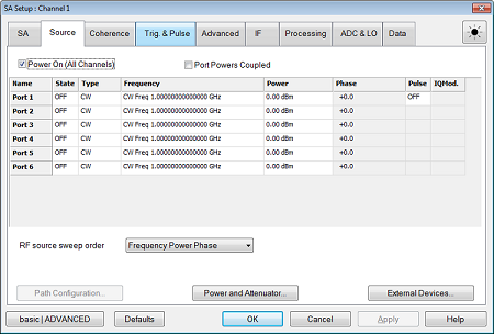
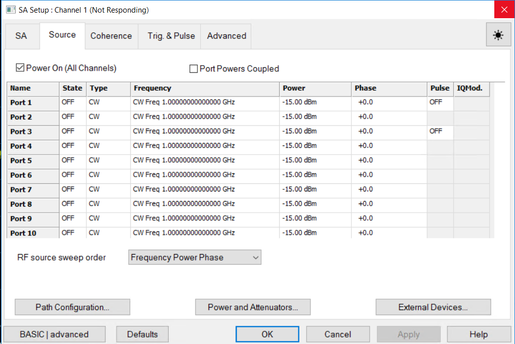
For M983xA, type or select independent attenuation values for each test port receiver. Set the attenuation value from 0 dB to 30 dB, 2 dB steps (Default value is 18 dB). Test receiver and reference receiver are coupled, per port.

SA Source Setup tab help

For M983xA,

Power On (All Channels)  Check to enable source power for all channels. Only turns power ON if the port State setting is ON.

Port Powers Coupled

• Coupled (checked)  The power levels are the same at each test port. Set power at any test port and all test ports change to the same power level.

• Uncoupled (cleared)  The power levels are set independently for each test port. Uncouple power, for example, if you want to measure the gain and reverse-isolation of a high-gain amplifier. The power required for the input port of the amplifier is much lower than the power required for the output port. A power sweep can also be performed with uncoupled power. Learn more about Setting Independent Port Power.

Source Cells

Name - Lists the test ports through which an internal source is available. If an external source has been configured, it will appear at the bottom of the list.

State

• ON  Source power is ALWAYS ON. Only one port can be turn on unless the unit has the second source or multi-module/unit configuration.   See also Setting Port Power On/Off for the Second source and Multi Module/Unit configuration.

• OFF  Source power is never ON, regardless of the measurement requirements. Use this setting to prevent damage to a sensitive DUT test port.

• No Control  Available ONLY on external sources. The SA application will NOT control the external source.

Type (Sweep)

CW - The source is set to a CW frequency.

LinFreq - The source is set to sweep from the Start to Stop frequency.

Power - The source is set to a power sweep.

Phase - The source is set to a phase sweep.

LinF+Pwr, Freq+Pha, Pow+Pha, Fr+Pw+Ph - Multi-parameter sweep for the specified parameters. Set the range of sweep for each parameter.

Frequency - Click in the cell, then click Edit, to start the Frequency Settings dialog (below).

Power - Sets the power level at the output of the source. Click in the cell, then click Edit, to start the Power Settings dialog (below).

Phase - Control source phase of a VNA source or external source.

Pulse - Enable/disable pulse measurements. Learn more.

IQMod. - Modulated I/Q file. Clicking Edit accesses a dialog for setting up an I/Q modulated file that is sent to a source for measuring Noise Power Ratio (NPR). Refer to the Noise Power Ratio (NPR) Settings topic for descriptions of the modulation dialogs.

RF source sweep order

Frequency Power Phase - Sweep from Start to Stop frequency first then sweep power then sweep phase.

Power Frequency Phase - Sweep power first then sweep from Start to Stop frequency then sweep phase.

Phase Frequency Power  - Sweep phase first then sweep from Start to Stop frequency then sweep power.

Phase Power Frequency - Sweep phase first then sweep power then sweep from Start to Stop frequency.

Frequency Phase Power - Sweep from Start to Stop frequency first then sweep phase then sweep power.

Power Phase Frequency - Sweep power first then sweep phase then sweep from Start to Stop frequency.

Buttons

Path Configuration (M983xA) Learn more

Power and Attenuator  Learn more

External Devices  Learn more

SA Coherence Setup tab help

Multitone

The set of Multitone properties enable an enhanced Image Rejection mode that takes benefits of the stimulus test signal knowledge.

If the stimulus test signal is repetitive with a repetition rate of x seconds, it only contains tones that are on a 1/x frequency grid. Example: if the test signal out of an arbitrary wave generator repeats every 1 ms, then it only contains frequencies on a 1 kHz grid (noise is not considered here). We will take this into account here to make the PNA-SA DFT analysis grid landing exactly on the same grid.

Moreover we will use the test signal knowledge to adjust the PNA-SA LO frequencies in order to avoid having 2 tones from the multitone stimulus signal landing at the same location at the PNA IF side. This makes the image rejection process deterministic.

Enable multitone image rejection

• Enabled (checked) The other parameters of the Multitone dialog are taken into account. Enabling this mode will set the DFT mode to arbitrary, the RBW shape to No Window, the RBW grid to a set of suitable values, and the list of analysis LOs accordingly. This setting is not compatible with the advanced settings “Force ADC record size” or “Force LO to frequency”.

• Disabled (cleared) Legacy stochastic image rejection mode of the PNA-SA application. When disabled, the window type is set back to what it was before enabling, and the RBW list is also set to the previous setting.

Tone Spacing - The tone spacing of the multitone signal (Hz).

Waveform Period – 1 over the tone spacing. This is the test signal repetition rate (seconds).

Reference Tone – If the multitone grid does not start from 0 Hz, its offset is set here. To make this more convenient, this dialog accepts as well the frequency of any tone of the multitone grid (Hz).

Reject up to harmonic – Set the number of test signal harmonics you want to be protected against. This adds constraints to the list of LOs used to cover the span.

Nyquist protect order – Enhancement for the deterministic coherent image reject mode. It ensures the Nyquist images of the signal tones in the IF bandwidth are not falling back on top of real signal frequencies. To be able to enable Nyquist protection, the tone spacing of the coherent signal cannot be an integer divider of the ADC sampling clock (100MHz for a PNA). Enabling this option often results in a larger ADC recordsize (or a smaller DFT tone spacing) at SA receiver side.

Vector Averaging - Average ADC samples by the specified number (≥1) in FPGA memory before the DFT processing. For example, if an ADC record size of 1,000 samples is acquired and Vector Averaging is set to 2, then 1,000 samples will be averaged to 1,000 samples and the result (1,000 samples) will be stored in FPGA memory. In other words, we acquire 2,000 samples form ADCs and send 1,000 averaged samples to the next processing stage. Vector averaging helps to reduce noise and increase dynamic range. However, this feature should only be used when the stimulus frequencies are known and coherent with the current ADC record size. A value of 1 means no averaging. Note this feature behaves like ADC Stacking+1. The maximum vector averaging value is 65536 or below. It depends on the RBW and the decimation.

Check box- Check to enable the ADC sample Vector Averaging to be specified manually.

Note: Vector Averaging and Video Bandwidth averaging cannot be set together. When enabling vector averaging, if the coherent mode is enabled then Video Bandwidth is turned off . The ADC Record Size x Vector Averaging must be ≤ 64 Mega Samples (or ≤ 32 Mega for some multiple receivers configurations).

Note: Vector Averaging is a great averaging method when Coherent Multitone mode is enabled. We recommend increasing it in Coherent Multitone mode instead of reducing the RBW to reduce the noise floor.

Note: Coherent mode (and Vector Averaging too) will work well if and only if the signal source and the PNA have their reference clocks synchronized. This is usually done by connecting a 10 MHz reference BNC cable between the signal source and the PNA.

Note: Vector Averaging is also known as Stacking. In fact, Vector Averaging = stacking +1.

Data Display

• Show All - Legacy behavior, shows the noise or the spurious between the tones. Note the RBW shape for multitones (No Window) makes the noise or the out of grid spurious amplitude values not accurate.

• Zero the non-tones - All the span frequencies that are not on the multitone grid have their amplitudes set to -200 dBm before correction. This makes band power marker measuring only the power for multitone frequencies, and not the noise power.

• Discard the non-tones - Deletes span frequencies that are not on the multitone grid.

Multitone settings are valid - Displays status of multitone settings.

Tone Phases and Phase Stitching

Compute Phases - Check to enable phase computation.

Note: In the SA tab, Detector Type muse be set to Bypass to compute phases.

Display Phases if Tone Power > - Set the phase display minimum level.

Phase Stitching

Phase stitching is performed for wide band signals to maintain phase continuity across the entire span when running the SA coherent mode with Compute Phases enabled. Wide band signals use many LO acquisitions across the span. Each LO has its own phase and each RF frequency is seen by two LO acquisitions. Phase stitching is performed from the energy in the overlapping area between two LO acquisitions. If energy exists in the two LOs, the phase of the first LO is measured, then the phase of the second LO is measured, then phase correction is performed. This is repeated across the entire span to maintain phase continuity.

Note: The Image Reject Type in the Advanced tab must be set to Min, LO High (2 overlaps on same IF side) for wideband phase stitching.

Enable Phase Stitching from HW timestamps - Enables/disables phase stitching using hardware time stamps to determine the phase of each LO acquisition and stitch them back together with phase consistency. Compute Phases must be enabled.

Enable Phase Stitching from overlapped areas - Enables/disables phase stitching across the entire span.

Stitch Phases if Tone Power > - If power in the overlapping areas between 2 LOs is below a specified level, then phase stitching will not be performed between these 2 LOs. It is still performed in other areas if there is enough energy. This ensures that noise is never used for phase stitching.

Receiver for Stitching - This function is used to manually select a receiver for phase stitching.

Auto - Check to allow the receiver used for phase stitching to be selected automatically. Multiple receivers can be involved in a measurement but the one with the highest energy in the overlap area is used for phase stitching. This receiver selection is performed independently for each overlapping area across the RF span.

IQ data generation

Compute time domain IQ - Enables/disables computing time domain IQ.

Auto Fill IQ settings button - Fills in the IQ settings automatically. Keep whole sweep data (Processing tab), Compute time domain IQ, Enable multitone, and Compute Phases (Coherence tab) must be enabled before selecting the Auto Fill IQ settings button. If the settings are valid, the Valid IQ Settings under Info (Processing tab) displays OK. Time domain IQ will not be computed until the IQ settings are valid.

Receivers - The receiver list can be either ALL, or a specific valid receiver. This selection determines which receiver data will be transferred to the 89600 VSA.

IQ keeps aligned with SA center, span, coherence - Check to recompute the advanced IQ parameters (IQ center, IQ sample rate, IQ number of points) automatically if a SA sweep parameter change is performed.

VSA Setup... button - Accesses the VSA 89600 Link Setup dialog for connecting the VNA to the VSA. Refer to the Link VNA to 89600 VSA topic for information.

Trig. & Pulse Dialog tab help

Trigger... - Accesses the Trigger dialog for setting up triggering.

Hold - The channel accepts NO trigger signals.

Single - The channel accepts ONE trigger signal, then goes into Hold.

Continuous - The channel accepts an infinite number of trigger signals.

Pulse Measurements

Off - Turns pulse off.

Standard Pulse - Turns pulse on.

Duty cycle - Displays the duty cycle relative to the current settings for Pulse Period and Pulse Width (Pulse Width/Pulse Period).

Meas. Width - Sets the time the measurement pulse is on.

Pulse Period pulldown - Allows the selection of the following:

Pulse Period - The time to make one complete pulse.

Pulse Frequency - The reciprocal of Period (1/ Period).

Pulse Duty Cycle - Pulse Width divided by the Pulse Period.

RF Pulse Width - Sets the width of the RF Source pulse.

One LO Acquire - The ADC acquisition time required to measure the data for a single FFT.

Full Sweep - Complete cycle time of measurement including background sweeps.

Pulses per LO - Number of pulses which will occur during the sweep for each LO.

Pulse Details

Name - Pulse generator outputs in numerical order.

Device -  Indicates the device being controlled by the pulse generator output.

• Pulse0 - Always set to Receiver. Sets the amount of time to wait before triggering the ADC to begin acquisition and is always selected for Pulse0 and cannot be changed. Pulse0 adds (ADC Delay) + (Modulator Delay). The ADC will begin measuring data 250 ns before the rising edge of Pulse0. This delay is indicated in the Fixed ADC Delay = 250 ns annotation.

• Pulse1 through Pulse4 - Pulse outputs can be set to the following:

• • RF Src - Selecting RF Src indicates that the pulse signal is used to drive the RF modulator. Only one pulse generator output can be used to drive an RF source. If you try to set more than one pulse generator output to RF Src, then the other one will be set to User N (where "N" is the pulse generator number).

  • User 1, User 2, User 3, User 4 - Labels for user convenience. These labels do not connect the pulse generator to any specific hardware. These selections may be used to control a DUT, DC biases, or other signals.

  • Activity - This selection outputs a signal on Pulse4 when the ADC is active. This is the same as Pulse4 Output Indicates ADC Activity on the Pulse Generators Setup dialog. If ADC is selected for Pulse4, then the pulse width and delay entries are grayed out because Pulse4 is no longer a pulse output.

Width - RF Source pulse width. This setting is the same as Pulse Width under RF Pulse.

Meas Delay - Sets the time before each pulse begins.

Width Adjust - Adjusts the measurement pulse width.

Invert - Check to cause the pulse ON time to be active low and OFF to be active high.

Enable - Check to enable individual pulse generators.

Plot Pulse Timing... - Accesses Pulse Timing display to evaluate the pulse timing setup.

Pulse Generators... - Accesses the Pulse Generator Setup dialog for setting up pulse measurements.

Advanced Settings Dialog tab help

Properties

RBW Shape - Selects the digital filter (window) to apply to the time domain IF signal. The filter effectively "shapes" the signal before application of the DFT to help avoid discontinuities which add unwanted frequency content to the spectrum. Each filter has its own advantages and disadvantages.

Gaussian - Selects a Gaussian window. The Gaussian window has good frequency separation and moderate amplitude accuracy. This window provides higher dynamic range because it has much lower side lobes. It is used for general-purpose measurements and when high dynamic range is required.

Flat Top - Selects the flat top window for amplitude measurement of sinusoidal frequency components. The flat top window has moderate frequency separation and excellent amplitude accuracy. It is typically used for narrowband signals when measuring the amplitude of a particular frequency component with greater amplitude accuracy.

Kaiser - Selects the Kaiser window which is an approximation of a Slepian window using Bessel functions. This window has a relatively high dynamic range and is similar to the Blackman window.

Blackman - Selects the Blackman window. This window has a relatively high dynamic range and is similar to the Kaiser window.

No Window - The No Window selection does not modify the time-domain data in any way before applying the DFT. This selection is very fast but may yield a significant number of side lobes in the frequency domain because of spectral leakage. This selection has a rectangular shape and does not attenuate any portion of the time record.

Image Reject Type - Sets the minimum number of distinct DFT acquisitions to use when computing an actual signal. As the number of DFT acquisitions increases from the None, LO Low setting to the Max setting, an increased number of erroneous signals are eliminated. Therefore, the Better and Max settings provide the highest confidence that what remains are actual signals, at the expense of slower measurements.

None, LO High - Selects 1 acquisition with the LO higher than the receiver frequency.

Note: Selecting None, LO High with full span is not possible. See SA Warning Messages.

None, LO Low - Selects 1 acquisition with the LO lower than the receiver frequency.

Note: Selecting None, LO Low with full span is not possible. See SA Warning Messages.

Min - Selects 2 acquisitions.

Min, LO High - Selects 2 acquisitions (like Min) and both acquisitions consider that the LO is higher than the receiver frequency.

Min, LO Low- Selects 2 acquisitions (like Min) and both acquisitions consider that the LO is lower than the receiver frequency.

Normal - Selects 4 acquisitions.

Better - Selects 6 acquisitions.

Max - Selects 8 acquisitions.

Image Reject Strength - Sets the image rejection strength. During the image rejection process, several LO acquisitions overlap at the same RF frequency (depending on the Image Reject Type). As a result, different RF signal values can be returned. This feature sets the acceptable power differences between measurements performed with different LOs in determining actual signals. Possible values are Weak, Normal, Strong. Weak accepts more difference between measurements, and strong less difference.

Auto RBW/VBW - Sets the ratio of Resolution Bandwidth to Video Bandwidth when the Video Bandwidth is in Auto mode.

Span/RBW - Sets the ratio of Span to Resolution Bandwidth when the Resolution Bandwidth is in Auto mode.

CF Step Size - Manually sets the amount Center frequency change that occurs when ▲|▼ is clicked (next to the value).

Auto - Each press of the ▲|▼ arrows increments or decrements the Center frequency by 5% of the current frequency span.

Occupied BW search min - Sets the minimum search frequency to use during an Occupied BW search measurement. Power below this frequency is ignored. See Occupied BW Ratio for information about setting up this measurement type.

DC Sources

DC source control allows the spectrum to be measured at multiple DC source settings.

Enable DC Outputs - Enables all DC source outputs that are turned ON in the DC Source dialog. This same selection is found in the DC Source Dialog.

Enable DC Sweep - Enables the DC sources to sweep between their start and stop voltages. If not selected, then the DC sources will be set to their start voltages.

Number of DC levels - Defines the number of voltage levels in the DC sweep.

The following settings apply to the measurement loop order. The SA may be programmed to loop through a series of spectrum measurements at multiple RF source frequencies, multiple RF source powers, and multiple DC voltages. These radio buttons determine whether the DC sources are swept before the RF power and frequencies are swept, or whether the DC sources are swept after the RF power and frequencies are swept.

Sweep Order

DC before RF - Sweep through each DC voltage step first then sweep through the next frequency.

RF before DC - Sweep through each frequency step first then sweep through the next DC voltage.

External Devices... button - Learn more.

DC Sources... - Configure internal DC sources. Learn more.

Frequency Converter Dual-Band Setup

The dual band configuration adds support for frequency conversion measurements. The following shows a down-converter measuring lower and upper ACPR and NPR. For this example, the RF input is 3.1 GHz on Port 1 from an N5182A MXG, the mixer IF output is 2.2 GHz on Port 2, and the mixer LO input connected to Port 4 is 900 MHz.

Note: The frequency conversion measurements also supports power sweep types to sweep from a start to a stop power.

Enable Frequency Converter Configuration - Automatically configures separate segment sweeps to display both input and output signals regardless of the frequency separation. In the above down-converter example, the segment sweep for the output (signal on the left) was set to 2.04 GHz to 2.36 GHz while the input segment sweep (signal on the right) was set to 2.94 GHz to 3.26 GHz. This was configured automatically when the check box is checked.

Sweep mode - Three selections are available with or without Acquire all receivers checked:

Both bands - Sweep both input and output bands

Input band - Sweep input band only.

Output band - Sweep output band only.

Acquire all receivers - This selection determines whether to measure all receivers or stop measuring all receivers.

Port - Selects the port number to assign to the input and output.

Source - Selects RF signal source from the pull down menu.

Center - Sets the center frequency of each band.

Inverted spectrum - Enable or disable inverting the spectrum (or mirror) by the frequency converter operation. The inverted information allows for proper setting of markers (band power, NPR, ACPR, etc.).

Advanced >> button - Accesses the IF, Trigger, Processing, ADC & LO, and Data dialogs.

IF Dialog tab help

IF Gain

Auto - Selects the appropriate amount for gain versus RF frequency bands for each receiver IF Path.

Or select a specific amount of gain (in dB) for IF receiver paths.

Couple all IF paths - When checked, all receivers assume the same setting. When cleared, each receiver can assume an individual setting.

IFConfig - Accesses the IF Path Configuration dialog. Learn all about IF Path Configuration.

IF Bandwidth

DFT Bandwidth Auto - Enables the default values for DFT bandwidth.

With Auto checked, the default values are:

Wide - 1 MHz to 30 MHz

With Auto unchecked, the values can be entered manually. The ranges are:

Wide - 500 kHz to 44 MHz

Processing Dialog tab help

DFT Type - Sets the DFT record size type. The types include:

Power of 2 - Sets the DFT record size to the next power of 2 greater than or equal to the current ADC record size. This is the fastest DFT processing available; the power of 2 record size allows for very efficient computation shortcuts (also known as the FFT algorithm).

Fastest - Sets the DFT record size as close as possible to the ADC record size (larger or equal) while optimizing processing speed.

Optimized Radix - Sets the DFT record size to the minimum integer number larger or equal than the ADC record size that can be decomposed with 2,3,5,7,11,13 radixes (also known as the 13-smooth numbers). The Intel CPUs have shared-coded trigonometric values for 2, 3, 5, 7,11, 13 fractional angles; the DFT code takes benefits from that for efficient DFT processing.

Arbitrary - Sets DFT record size equal to the ADC record size. If the current ADC record size is a large prime number, then the DFT can be very slow. Sometimes, the record size will be increased more than the minimum number required to match the 13-smooth condition, if the whole processing of the sweep is faster with a record size that has a faster DFT time. There is a trade-off here: increasing the record size to speed up the DFT will increase the amount of data to process for the further steps of the SA processing (image rejection, detection).

Additional comments:

There is a given ADC record size that gives a given RBW (for a given window type), the RBW evolves as 1/ADC record size. If the DFT record size must be greater, depending on the DFT mode, some zeros will be added to the ADC record size. This is the difference that can be noted between the ADC record size and the DFT record size on the Advanced Processing dialog.

When running the coherent mode of SA, the Arbitrary mode will always be selected, to make sure the DFT bins frequencies exactly land on the coherent signal tones.

The Power of 2, Optimized Radix, and Fastest mode have the same behavior regarding the RBW setting: These 3 modes are increasing the ADC record size to the next best match. This is more sensitive with Power of 2 mode, as the density of available ADC record size is sparse.

The Power of 2 mode makes the SA computation behave exactly like some tools based on FFT processing; this is a use case of this mode. The other use case is to get the fastest processing time that can be useful for intensive spurious search measurements. The penalty is the small number of RBW values available.

The Optimized Radix mode is currently the default mode, this is the one that gives the most accurate RBW setting. The Fastest is to be tried if speed matters for a given non-coherent SA setting.

For example: running 100 kHz RBW with Gaussian filter, the ADC record size must be 1988 samples. Here are the DFT lengths for the different algorithms:

End of Sweep Processing

The End of Sweep Processing function is used to keep the memory buffer of the last full sweep in memory for further processing. This is not done by default because keeping the whole data in memory requires large amounts of memory and processing (for example, in the case of wide span or low RBW).

Before the implementation of this function, raw data could be sent to a file (ascii or binary) or the fifo, as this can be done while sweeping with no need to keep the whole data in memory. This option is still available.

With each sweep, the data buffers are filled, and are erased if a new speed is started. In other words, this feature works well in the logic of “Single” sweep. You must ensure that a full sweep is in the buffers before pulling out raw data.

Receivers - The receiver list can be either ALL, or a specific valid receiver. Only the receivers currently defined for measurement traces can be kept in memory.

Keep whole sweep data - Check to keep last full sweep data in memory.

IQ generation parameters

IQ Carrier Frequency - Sets the IQ carrier frequency.

IQ Sample Rate - Sets the IQ sample rate.

Number of IQ Pairs - Sets the number of IQ pairs.

Info

Acq. Time for 1 LO - Displays the LO acquisition time which is the ADC Record Size x ADC Sampling Frequency (10 nsec or 40 nsec) x (1 + Stacking) x (Video Averaging Coefficient). When settings affecting this value are changed, the displayed value is not updated automatically and will become grayed out. To update the value, close then open this dialog. The analyzer must be sweeping to update values.

Span Acq. Time - Displays the total acquisition time to perform a SA sweep. For simple cases, it is the acquisition time of one LO multiplied by the number of LOs. When running Multiple recording coherent pulse mode, the acquisition time here takes into account the duty cycle of the pulses.

Span LOs count - Displays the number of LO acquisitions determined by the Image Reject selection and the span. When settings affecting this value are changed, the displayed value is not updated automatically and will become grayed out. To update the value, close then open this dialog. The analyzer must be sweeping to update values.

Span bins count - Displays the current span DFT bin count, the number of DFT points processed across the total RF span. When the Detector is bypassed, this is the number of points that are sent to the display.

DFT resolution - Displays the DFT resolution.

DFT record size - Displays the current DFT record size.

ADC record size - Displays the ADC record size value.

ADC with average - Displays the ADC acquisition time of one LO multiplied by the averaging (vector averaging or video averaging) factor. It is the straight ADC acquisition time that has to go into the ADC memory for further processing.

ADC frequency - Displays the ADC frequency.

Coherence ratio - Displays the coherence ratio value.

IQ record duration - Displays the current duration of the IQ record.

VSA IQ pairs count - Displays the number of IQ pairs transferred to the VSA.

Valid IQ Settings - Displays whether the IQ settings are valid or not. If valid, OK is displayed.

Display image reject traces - Check to display the data acquired by each LO. The minimum number of meaningful traces is determined by the "Image Reject" setting (described in the Advanced dialog above).

About Image Reject Traces

These traces display the spectral content of the measured signal for each LO frequency used in the acquisition. The number of ImageReject traces you want to look at is tied to the 'Image Reject' setting. For example, 'Normal' setting is at least 4 ImageReject traces, and 5 more generally.

This function is intended to be used as a diagnostic tool if something looks suspicious.

Note: Mixer calibration and user calibration are not applied to the image rejection traces, thus the amplitude readout value is not accurate.

About Acquisition Time and Sweep Time

The Acquisition time for 1 LO is really the duration of the ADC acquisition run for one LO setting. Depending on the SA span and the image rejection mode, the number of LOs required for a given SA frequency span changes. This number is reported as Span LOs count. So the total ADC acquisition time for a given span, aka Sweep Acq. Time, is the product of Acquisition time for 1 LO x Span LO count (unless Multiple Recording mode is running, then the Multiple Recording  multiplication factor is to be considered).

The entire sweep time is a significantly larger number than the Sweep Acq. Time. Each time the LO is moved, there is a settling time required for LO stabilization. Then each time some raw ADC data is acquired, there is some time to move the data across the buses (the data amount is multiplied by the number of ADCs at work, when several RF receivers are acquired). All the further processing (windowing, DFT, IF calibration, Image Rejection, User calibration) is CPU time consuming, the lowest the RBW the more time it takes to process the DFT samples (there are more DFT samples).

The Image Rejection mode MIN instead of Normal (when not running coherent mode) is a popular way to speed up the sweep time, as roughly half of the LOs count is required, at the cost of higher likelihood of false spectrum spurious (but real signal spurious are still always detected).

The video averaging is digital, it runs several times the ADC acquisitions and windowing and DFT and then averages. The number of times this extra processing is done for video averaging is indicated at the Video averaging count at the SA main page.

When available, the vector averaging is done at the FPGA side, it multiplies by the averaging factor the ADC acquisition time, and it doubles the data amount across the data buses (32 bits instead of 16 bits ADC data representation). The following parts of the processing are not impacted, the quantity of data to process at host CPU side is not increased. Thus the vector averaging is a very efficient way to get lower noise floor with minimum additional CPU time.

The display processing is a very significant part of the sweep time. The number of display points can be set (defaults to 1001), then the code often has to do a data reduction to go from millions of DFT points to 1001 display points. This is the so-called detector processing. This process is CPU intensive, especially the Peak detector that recomputes an X-axis frequency grid each sweep to align each x-axis point to the local interpolated peak. FastPeak is less frequency accurate for the peak points positions but very significantly faster. If the span is narrow, bypassing the detector can speed up the sweep. Turning off the display is another option, it bypasses most detection and display algorithms, thus speeds up the sweep in remote programming modes.

The status bar of the channel shows the last measured SA sweep time, and if some settings are changed, the first sweep after a change shows an estimate with a ~ preceding the timing.

ADC & LO Dialog tab help

ADC Sampling

ADC Sample Frequency - Select between 100 MHz and 25 MHz.

Auto - Check to automatically set the ADC Sampling Frequency.

Enable FIR for 25 MHz - Enables the FIR filter for 25 MHz decimation: reduces the noise floor.

Overrange warning percent - Sets the percentage of the ADC input full scale. SA sweeps require thousands (or millions) of ADC samples processed by the FFT. The maximum ADC sample value is kept for the whole sweep, as it is an image of the peak voltage in the IF chain of the instrument. Instead of calibrating this value to Volts, a percentage value of the ADC input full scale is used. If the value is too high, reduce the IF gain or add RF attenuation to maintain the linearity of the instrument. If the value is too low, the signal amplitude to too low and under-utilizing the ADC range. Increasing the IF gain may increase the measurement quality (reducing the noise floor).

Show ADC Ranges... - Displays the ADC ranges of the current receivers from the last sweep if the Trigger mode is currently on Hold.

ADC Raw data

Force ADC record size - Sets the ADC record size which is dependent on the Resolution Bandwidth and ADC Sampling Frequency:

Check box - Check to enable the ADC record size to be specified manually. Doing so sets the resolution bandwidth. The size range is 64 Samples to 32 or 64 MegaSamples depending on the selected receivers. The DFT size will be recomputed accordingly to the DFT Type setting. When not checked, the value displayed is the current ADC record size. This feature is not compatible with Coherent Multitone mode.

Stacking - Stack ADC samples by the specified number (≥1) and store result in memory. For example, if an ADC record size of 1,000 samples is acquired and Stacking is set to 1, then 1,000 samples will be added to 1,000 samples and the result (1,000 samples) will be stored in memory. In other words, we acquire 2,000 samples form ADCs and send 1,000 stacked samples to the next processing stage. Stacking helps to reduce noise and increase dynamic range. However, this feature should only be used when the stimulus frequencies are known and coherent with the current ADC record size. A value of 0 means no stacking.

Check box- Check to enable the ADC sample stacking to be specified manually.

Note: Stacking and Video Bandwidth averaging cannot be set together; Video Bandwidth has precedence. The ADC Record Size x (Stacking + 1) must be ≤64 Mega Samples.

Note: Stacking is a great averaging method when Coherent Multitone mode is enabled. We recommend increasing the stacking in Coherent Multitone mode instead of reducing the RBW in order to reduce the noise floor.

LO

Randomized LO - Check to allow dithering of the LO values used when taking a sweep. Allowing randomized LO makes it less likely that erroneous signals will appear in the final measurement.

Force LO to Frequency - Sets the LO to a specified frequency. This check box can only be set if Image Reject is set to None, LO Low or None, LO High or Enable baseband X-axis mode (LO independent sweep) is checked.

Check box - Check to enable the LO frequency to be specified manually.

This function allows the LO source to be used mostly like another source that can be set up relative to a source port. For example, if Port 1 in the Source tab is set to a frequency of 1 GHz and the Force LO to frequency is set up as shown below, then the LO will track 1 MHz after the Port 1 source frequency.

Data Dialog tab help

Data Format -

Float LogMag (dB) - Sets the data format to log magnitude in dBm.

Float LinMag - Sets the data format to linear magnitude in volts.

Integers - Sets the data format to Packed Integers (each value is a short 16 bit integer, the equation to compute the dBm value is: dBm = Xshort/200.0 - 36.165.

Export receivers - Select the data to export from a specific receiver or all receivers.

Don't save data below threshold - Set data level threshold mode and threshold level in dBm. For text file output with verbose mode, only the frequencies with power greater than this threshold setting will be written to the file.

DFT bins count - Displays the current DFT bin count, the number of DFT points processed across the total RF span. When the Detector is bypassed, this is the number of points that are sent to the display.

Receivers count - Displays how many receivers are currently being exported. The number here can be less than the number of receivers specified in Export Receivers, if some of them at not selected in the channel.

Export to binary file - Set data to be exported to a binary file. Data is not exported until the next new sweep occurs.

Export to text file - Exports data only. Data is not exported until the next new sweep occurs.

Verbose mode - Exports frequency and data. Data is not exported until the next new sweep occurs.

Erase files each new sweep - Selecting this option will erase the data after each sweep. If this option is not checked, the data from each sweep will continue to be appended to the output data file which can create a very large file size (and fill the disk, with many unwanted consequences).

File name prefix - The receiver selected in Export receivers will be appended to the prefix name specified in this field with either ".txt" if a text file is exported or ".bin" if a binary file is exported. For example, if C:\Temp\SA_DATA_OUT is entered into the File name prefix field and the "B" receiver data is exported to a text file, the data will be exported to a file called SA_DATA_OUT_B.txt.

Record size (bytes) - This is the byte size of binary data output.

Export markers with data files - Adds marker data and data to the text file (*.txt) output.

Export all markers to a single file - Adds all marker data to a single text file (*.txt) output.

Export to FIFO buffer - Exports data to the FIFO (First-IN, First-OUT) data buffer. FIFO is a circular buffer that allows very fast Read-Write access.

Export to shared memory - Exports data to shared memory (Microsoft Windows feature) which is the fastest way to transfer data between applications. The application that is retrieving data has to register itself to Microsoft Windows with the same share name.

Share name - Assigns a specified name to the shared data.

Export IQ data

Export to binary file - Enables/disables the IQ data to be output to a binary file (*.bin).

Export to text file - Enables/disables the IQ data to be output to a  text file (*.txt).

(Source) Frequency Settings dialog help

In the SA Setup Source Tab (above):

> When (Sweep) Type = CW, set the CW Frequency.

> When (Sweep) Type = Linear, the following dialog appears:

Settings

Sets the source frequency range. Use either of the following pairs of settings to set the frequency range.

Start /Stop - Specifies the beginning and end frequency of the swept range.

Center /Span - Specifies the value at the center and frequency range.

Source Number of Steps - Sets the number of steps the source will make across the specified source frequency range.

SA Sweeps / Source Step - Sets the number of SA (receiver) sweeps for each Source Step. This setting is common to all sources.

(Source) Power Settings dialog help

In the SA Setup Source Tab (above):

> When (Sweep) Type = CW, or LinFreq, the following dialog appears:

> When (Sweep) Type = Power or LinF+Pwr, the following dialog appears:

Settings

Sets the source power range. Use either of the following pairs of settings to set the power range.

Start /Stop - Specifies the beginning and end power of the swept range.

Center /Span - Specifies the value at the center and power range.

Source Number of Steps - Sets the number of steps the source will make across the specified source power range.

SA Sweeps / Source Step - Sets the number of SA (receiver) sweeps for each Source Step. This setting is common to all sources.

How to select and configure Measurement Parameters

Using Hardkey/SoftTab/Softkey

Using a mouse

1. Select a trace by pressing Trace > Trace N >  Trace N.

2. Press Trace > Trace Setup >  Measure....

3. Select a parameter.

1. Right-click on a trace.

2. Select a parameter

How to Configure a Second Source

Using Hardkey/SoftTab/Softkey

Using a mouse

1. Press Macro > Macro1 > SA Multi-module Cal

1. Click Utility

2. Select Macro

3. Select SA Multi-Module Cal

SA Multi Module Calibration dialog box help

Take Calibration: Starts calibration sequence. All ports should be open

Calibration Status: Show the calibration status. Calibration is enabled only when the calibration data exists.

Calibration On Enable/disable the multi module calibration.

Note: The calibration data is stored in your controller. When you change the controller, re-calibration is required.

Note: System > System Setup > Remote Control > Hislip must be enabled before the execution. The hislip address must be set at 0.