The N100A DCA-X and DCA-M series modules are sampling oscilloscopes. Understanding the differences between sampling oscilloscopes and traditional real-time oscilloscopes will help you get the most benefit from your measurements. In this topic you'll learn that sampling oscilloscopes:

• Require an external trigger signal that is synchronous with the input data.
• Must be armed with an input channel turned on in order to respond to a trigger.
• Include a delay between the time when the oscilloscope responds to a trigger and when the oscilloscope is armed and able to respond to another trigger.
• Include a minimum time delay occurs between the time a trigger is received and when the data is actually sampled.
• Displayed waveforms consist of many sampled points, and each sampled point requires a trigger event (edge).

Oscilloscopes Compared

Real-Time Oscilloscopes

A real-time oscilloscope, sometimes called a “single-shot” scope, captures an entire waveform on each trigger event. Put another way, this means that a large number of data points are captured in one continuous record. To better understand this type of data acquisition, imagine it as an extremely fast analog-to-digital converter (ADC) in which the sample rate determines the sample spacing and the memory depth determines the number of points that will be displayed. In order to capture any waveform, the ADC sampling rate needs to be significantly faster than the frequency of the incoming waveform. This sample rate, which can be as fast as 80 GSa/s, determines the bandwidth which currently extends to 63 GHz.

The real-time scope can be triggered on a feature of the data itself, and often a trigger will occur when the incoming waveform’s amplitude reaches a certain threshold. It is at this point that the scope starts converting the analog waveform to digital data points at a rate asynchronous and very much unrelated to the input waveform’s symbol rate. That conversion rate, known as the sampling rate, is typically derived from an internal clock signal. The scope samples the amplitude of the input waveform, stores that value in memory, and continues to the next sample as illustrated in Figure 1. The trigger’s main job is to provide a horizontal time reference point for the incoming data.

Sampling Oscilloscopes (DCA-X/DCA-M)

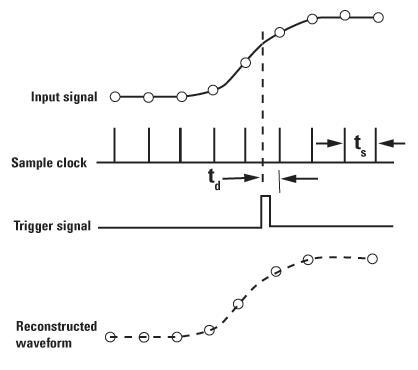
In contrast to the real-time scope, an equivalent-time sampling oscilloscope, sometimes simply called a “sampling scope,” only samples the input signal once per trigger. The next time the instrument is triggered, a small delay is added and another sample is taken. This incremental delay time is determined by the time base setting and the number of sample points. The intended number of samples determines the resulting number of cycles needed to reproduce the waveform. The measurement bandwidth is determined by the frequency response of the sampler which currently can extend beyond 80 GHz.

The triggering and subsequent sampling of DCA-X/DCA-M instruments is different from a real-time oscilloscope. The DCA-X/DCA-M:

• Require an external trigger signal that is synchronous with the input data. The oscilloscope can not synchronize directly to the signal being measured. You can also provide a trigger using a hardware clock recovery module.
• Must be armed with an input channel turned on in order to respond to a trigger. The oscilloscope is armed when it is in the run mode or in single acquisition mode (press the oscilloscope's Stop Single button). Press the button repeatedly to rearm the oscilloscope.
• A delay occurs between the time when the oscilloscope responds to a trigger and when the oscilloscope is armed and able to respond to another trigger. This delay (re-arm or setup-and-hold time) is on the order 25 μs. Therefore, while the rearming process occurs, many ignored trigger events can occur.
• Displayed waveforms consist of many sampled points, and each sampled point requires a trigger event (edge). For example, if a waveform trace consists of 500 points, then the oscilloscope must respond to at least 500 trigger edges.
• A minimum time delay occurs between the time a trigger is received and when the data is actually sampled. This delay is on the order of 24 ns. Therefore, the signal at the trigger point (time zero) is usually not seen unless the data is delayed (through cable lengths/delay lines) relative to the trigger signal. You can change the amount of delay in the Timebase Setup dialog box.

There are two ways to trigger the DCA-X/DCA-M and each results in a different data viewing format; either a symbol stream or an eye diagram.

Viewing Bit Streams on DCA-X/M

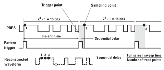
Viewing the individual UIs in the signal allows you to see the pattern dependencies in the system, but does not allow for high resolution with large numbers of UIs. In order to view a symbol stream, the trigger must only pulse once during the period of the input pattern and must be at the same relative location in the symbol pattern for each event. The input signal is then sampled and upon the next trigger event, the incremental delay is added and the symbol steam is sampled until the entire waveform is acquired. In order to view a symbol stream on the DCA-X/M, you must have a repetitive waveform; otherwise a real-time scope is needed. The triggering process to display a symbol stream waveform is shown in Figure 3.

Viewing Eye Diagrams on DCA-X/M

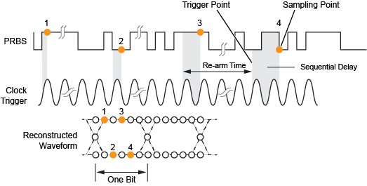
The other viewing mode is the eye diagram. This mode does not require a repetitive waveform and can help to determine noise, jitter, distortion, and signal strength among many other measurements. The eye diagram gives an overall statistical view of the system’s performance as it looks at an overlay of every combination of UIs in the symbol steam. The triggering required for this mode is a synchronous clock signal. At each trigger event, allowing for rearm time, the scope samples the data and builds the combination of all possible 1 and 0 combinations across the screen. Keep in mind the following points:

• Full rate clocks as well as divided rate clocks can be used for the trigger, however if the length of the pattern is an even multiple of the clock divide ratio, the eye diagram will be missing combinations and will therefore be incomplete.
• If the data is used as its own trigger, the eye diagram may appear complete, but the scope is only triggered on rising edges of the data pattern. This should be avoided to make accurate eye diagram measurements.

The triggering process to display an eye diagram is shown in Figure 4.

 

Repeating Square Wave Signal (DCA-X/M)

The following figure shows a square wave to be measured as well as the trigger signal.

The square wave to be measured is a 1 GHz signal. The DCA-X/M is configured to display 1001 points with a timebase scale of 100 ps/div (or 1000 ps across the full display). Therefore, the separation between points is 1 ps. When the DCA-X/M is armed, it is ready to respond to the first rising edge of the square wave. After this trigger event occurs, the first sample is taken. The minimum delay between the trigger event and sample point 1 is 24 ns.

The DCA-X/M then rearms and waits for the next trigger event. When the next trigger is received, the delay between the trigger event and the sample for point 2 is 24 ns plus an additional 1 ps. The second sample is taken from a different location in the waveform, but its time position is precisely located relative to the trigger event. Thus when the samples are displayed on the screen, the first and second sample (and the 999 subsequent samples) are placed precisely 1 ps apart. The waveform is precisely reconstructed from samples taken at many separate locations of the waveform. The samples are not taken from many points sampled in one section of the waveform. This sampling and acquisition process illustrates the requirement for the waveform to be repetitive in order for the sampling scheme to be valid.

Random, Non-Repeating Data Signal (DCA-X/M)

The following figure shows a random, non-repeating data signal. The trigger signal is a clock signal operating at the symbol rate. The rearm and delay times described in Example 1 apply to Example 2. The waveform is a 2 GBd signal; the instrument is configured to display 1001 points with a timebase scale of 100 ps/div. The first sample is taken as shown. The second sample is taken after the rearm and delay.

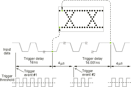
Due to the 25 μs rearm time, samples are acquired from arbitrary UIs in the data stream. However, the timing of all samples is precisely known relative to the synchronous trigger edge. The displayed waveform is a precise reconstruction of samples taken from many UIs in the digital waveform. The waveform is then a composite image of both high and low levels as well as the transitions between the two levels. This waveform is referred to as an eye diagram.

Non-Random Signal with Repeating Pattern (DCA-X/M)

The following graphic shows a digital waveform with a repeating pattern. It is not a random signal. The trigger signal is a pattern trigger. A pattern trigger is a signal that has a rising (or falling) edge that occurs only once per repetition of the pattern in a fixed position in time relative to the data pattern.

When the instrument is armed, it is ready to respond to the first trigger edge. After this trigger event occurs, the first sample point is taken. The minimum delay between the trigger event and sample point 1 is 24 ns. The instrument then rearms and waits for the next trigger event.

The second sample is then taken at a point in the pattern that is adjacent to the first sample point. Subsequent samples then follow continuously through a single section of the data pattern.

DCA-X Plug-in Modules

Plug-in modules have two measurement channels (optical/electrical, dual optical, or dual electrical) and provide sampling for the instrument. Most modules occupy one of two mainframe slots and can be installed in either the left (channels 1 and 2) or right (channels 3 and 4) slots of the mainframe. The 86107A precision timebase module and the 86108A precision waveform analyzer module (includes a precision timebase) both improve the jitter performance of the instrument. This improved performance allows the instrument to measure the true jitter of your signal. The precision timebase module can also be installed in either slot of the mainframe.