Interference Measurement Algorithm

Jitter Mode establishes a pattern trigger as described in Jitter Measurement Algorithm. When amplitude measurements are initiated by selecting to display an amplitude graph or table, the instrument uses the additional measurement algorithms in the order listed in this topic. To view a representative eye diagram showing the active sampling area, click the Graphs arrow to scroll up and hide the graphs.

You can adjust the measurement location of the sample area in Amplitude Measurements tab of the Configure Jitter Measurements dialog. By default, the measurement location is the center symbol position (50%) as measured between the symbol crossing points.

Measuring Inter-Symbol Interference (ISI)

Inter-Symbol Interference (ISI) is a measure of the pattern-dependent interference effects within a signal. It is a measure of how much the amplitude of a symbol depends on its location within the pattern.

The instrument uses the pattern trigger to step through the symbols in the pattern. The average amplitude of each symbol is obtained at the measurement location. The average level for each symbol is combined to build two ISI histograms: a histogram for the one level, and a histogram for the zero level. For each level, the peak-to-peak width of the histogram is reported as the ISI value in the Amplitude Table. A continuous running average of the average symbol level is maintained.

Measuring Random Noise (RN) and Periodic Interference (PI)

Random noise is uncorrelated to the pattern and assumed to follow Gaussian statistics. For each measurement cycle, a symbol is selected from which to acquire samples at the measurement location. One and zero data is kept separately. The deviation about the mean amplitude of this specific symbol shows the effect of uncorrelated noise and does not show the effects of pattern dependent noise components. This same uncorrelated noise is present on each symbol of the pattern. An RN/PI histogram is created from this data.

The periodic nature of the samples allows the noise values to be transformed into the frequency domain as can be seen on the Noise Spectrum graph. This results in a power spectral density of uncorrelated noise with the noise floor of the spectrum representing RN. The discrete frequency components, or spikes, represent the uncorrelated PI, which is a measure of the interference that is uncorrelated to the pattern, yet is periodic. After removing the uncorrelated PI spectral lines through interpolation, the remaining spectrum, which is the random components of noise, is integrated to determine the root mean square RN (rms) result which is listed in the Amplitude table.

The spectrum is not used to determine the uncorrelated PI. The instrument's maximum periodic sampling rate is 40 kHz, and any jitter spectral content that is above 20 kHz will be aliased. This limits the analysis of the noise spectrum to the noise floor and will not allow the periodic elements to be determined. The uncorrelated PI is instead determined from the RN/PI histogram that was used to determine RN. A dual-Dirac delta model is constructed using two identical Gaussian distributions. The width of each Gaussian is defined by the previously measured RN value. The separation between the peaks of the Gaussians represents the uncorrelated PI. The peak separation (PI value) is adjusted until the peak-to-peak width of the model matches that of the interference data histogram. Peak-to-peak width is defined to include 99.8% of the total area of the model or histogram. The resulting PI value is listed as uncorrelated PI ( δ - δ ) on the Amplitude table.

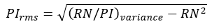
To calculate PI (rms), the variance of the RN/PI histogram is used in the following equation:

Measuring Deterministic Interference (DI)

At this point, the values for RN, PI, and ISI have been determined. Next, these values are combined to determine Deterministic Interference (DI) and Total Interference (TI). So far, probability density functions (histograms) have been determined for the uncorrelated noise (RN and PI) and for the correlated noise (ISI). The DI value is composed of both the ISI and the PI, but it is not a simple sum of the values, as each is defined by a statistical distribution. To determine the DI for the one level, the RN/PI and ISI histograms for the one level are convolved together and likewise for the zero level to create the Total Interference Histograms. These histograms are the probability density function of all of the measured noise, both correlated and uncorrelated. The dual-Dirac delta model methodology described above for extracting PI from the RN,PI histogram is applied to the total interference histogram. The same measured RN (rms) result describes the two Gaussian distributions, and the same fitting technique is used. The separation between the means of the two Gaussian distributions is listed as the DI (δ-δ) on the Amplitude table.

Measuring Total Interference (TI)

Total Interference (TI) is the width of the one (or zero) level distribution at a low probability or BER. TI is always measured at the same BER as the Total Jitter measurement. The BER value can be set in the Advanced tab of the Configure Jitter Measurements dialog. Click Measure > Configure Jitter Meas. The default value is 1E-12.

The tails of the total interference probability density function extend indefinitely. When there is a random noise component, a peak-to-peak value has meaning only when associated with a specific probability, which is found using the dual-Dirac delta model. The TI is determined by extending the dual-Dirac delta model down to the point where the probability of occurrence is less than 1 part per trillion (1E-12) of the whole. The width of the model at this threshold is listed as TI (1E-12) on the Amplitude table. TI values at other levels of probability can be obtained in a similar fashion.