Jitter Measurement Algorithm

When Jitter Mode is first entered, the oscilloscope automatically detects clock rate, pattern length, and trigger divide ratio from the trigger and input signals. (Automatic detection can be disabled.) The instrument then internally generates a pattern trigger. The pattern trigger occurs at an arbitrary relative symbol in the data pattern. Pattern trigger enables the oscilloscope to step through the pattern symbols and acquire all necessary data over a small range of timebase delay. The internally generated pattern trigger eliminates jitter that can be introduced by an external pattern trigger and eliminates errors induced by large ranges of timebase delay.

Edge Models

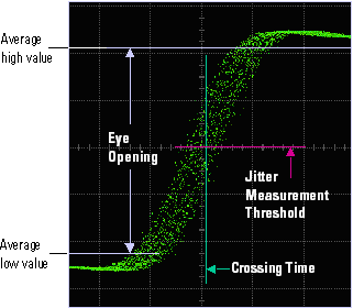
When Jitter Mode is entered or the Auto Scale button is pressed, the symbol-center times and crossing times (the transition times between low and high logic values) are determined. Crossing time data is sampled at a level midway between the average logic high value and the average logic low value. The average value for each logic level is measured at the symbol-center time. The sampled amplitude values are converted to jitter time values by means of edge models.

To view a representative eye diagram showing the active sampling area, click the Graphs arrow to scroll up and hide the Results graphs.

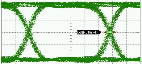
You can adjust the level of the sample area in the Jitter Measurements tab of the Configure Jitter Measurements dialog.

As the pattern trigger steps through the symbols, the FlexDCA applies averaging to remove any uncorrelated jitter components and then determines the average location of each edge. Because the sampling event occurs at the average location of the edge, an early arriving edge will have an amplitude above the middle, while a late arriving edge will have an amplitude below the middle level. To determine the amount of jitter on an edge from these amplitude samples, the amplitude-versus-time shape of the edge (known as an edge model) must be known.

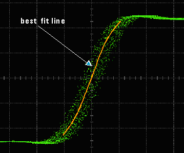
The oscilloscope builds edge models and uses these models as transfer functions to convert sampled edge amplitudes directly to jitter measurement values. Once the edge is modeled, every sample that is taken along the edge yields a jitter measurement.

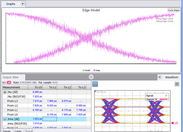
You can view the actual edge models used for a measurement by clicking Tools > Jitter Diagnostics > Edge Model Graph.

Two types of edge models are built: a single-edge model and 16 composite-edge models. Single and composite edge models are used to measure different jitter components. The single-edge model describes the amplitude-versus-time shape of a specific edge of a pattern and is constructed by taking 1024 samples across the entire span of one edge. A mathematical function is constructed that delivers the best fit, in a least squares sense, to the sampled data. The composite-edge models are very similar, except the samples used to construct these models are taken from multiple edges. Each composite-edge model is composed of 4096 points and is used to describe the amplitude-versus-time shape of a class of edges. A class is defined by the configuration of the four preceding symbols. For example, '00001' is one class of rising edge, and '00101' is another class. Similarly, '11110' is one class of falling edge, and '11010' is another class. Eight rising and eight falling edge classes are defined.

Correlated and Uncorrelated Jitter

After building the edge models, the instrument measures the jitter that is correlated to the data pattern, known as Data-Dependent Jitter (DDJ), and then measures the jitter that is uncorrelated from the data pattern. The uncorrelated jitter is made up of Random Jitter (RJ) and uncorrelated Periodic Jitter (PJ). Refer to the Jitter Components Tree to learn the relationship between the different types of jitter.

Measuring Correlated Jitter

To measure DDJ and its components, the pattern trigger steps through the pattern and takes samples from every edge. The composite-edge model associated with each edge's class is used to translate each amplitude measurement into separate jitter measurements for rising edges and falling edges. Probability-distribution-function histograms are created for the rising edge jitter, the falling edge jitter, and the combination of both rising and falling edges. These are shown on the Composite DDJ Histogram graph. The peak-to-peak spread of the histogram of all edges is shown in the DDJ Histogram graph and is listed as DDJ (p-p) on the R Jitter table. It is the arrival time difference between the earliest arriving edge and the latest arriving edge. The peak-to-peak spread of the rising edges or the falling edges, whichever is greater, represents jitter that is caused by Inter-Symbol Interference (ISI) and is listed as ISIJ (p-p) on the Jitter table. The difference between the mean of the rising edge positions and the mean of the falling edge positions represents jitter that is caused by Duty Cycle Distortion (DCD) and is listed as DCD on the Jitter table.

Sub-Rate Jitter (SRJ) is periodic jitter that is correlated to the data and has a frequency that is an integer sub-rate of the symbol rate. (Sub-rate x N = symbol rate.) This form of jitter is often associated with multiplexing data structures. For example, if one leg of a parallel data structure systematically results in a late or early edge, the jitter will be periodic in nature. It is correlated to the data stream, but may not be seen systematically on the same symbols in a given pattern depending on the relationship between the pattern length and MUX size. Another common source of SRJ is coupling of a sub-rate reference clock onto the full-rate data stream. Extraction of SRJ is complex, as SRJ can show up as DDJ when the pattern length is a multiple of any clock divisor used to trigger the instrument. Otherwise SRJ shows up as PJ.

Measuring Uncorrelated Jitter

An edge's deviation about its mean position shows the effect of uncorrelated jitter and does not show the effects of pattern dependent jitter components. This same uncorrelated jitter is present on each edge of the pattern. For each data acquisition cycle targeted at uncorrelated jitter, the instrument acquires all of its samples on a specific edge within the pattern, thus removing all pattern dependent jitter from the data. The single-edge model is used to convert amplitude samples to jitter values as samples are taken specifically at the edge. Subsequent acquisitions are taken from other edges in the pattern, but each individual acquisition record uses data from a single edge. Jitter data from all acquisitions is accumulated in the RJ,PJ Histogram graph. The periodic nature of the samples allows the jitter values to be transformed into the frequency domain. This results in a power spectral density estimate of uncorrelated jitter. The noise floor of the spectrum represents RJ. The discrete frequency components, or spikes, represent the uncorrelated PJ. After removing the uncorrelated PJ spectral lines through interpolation, the remaining spectrum, which is the random components of jitter, is integrated to determine the root mean square RJ (rms) result, which is listed on the jitter measurement Jitter table; this is the standard deviation of the random jitter distribution.

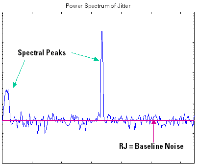
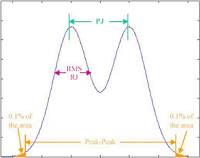
The spectrum is not used to determine the uncorrelated PJ. The maximum periodic sampling rate of the N1000A is up to 250 kHz (86100D is 40 kHz), and any jitter spectral content that is above 125 kHz will be aliased (20 kHz on 86100D). This limits the analysis of the jitter spectrum to the noise floor and will not allow the periodic elements to be determined. The uncorrelated PJ is instead determined from a histogram of the jitter data that was used to determine RJ. A dual-Dirac delta model is constructed using two identical Gaussian distributions. The width of each Gaussian is defined by the previously measured RJ (rms) value. The separation between the peaks of the Gaussians represents the uncorrelated PJ. The peak separation (PJ value) is adjusted until the peak-to-peak width of the model matches that of the jitter data histogram. Peak-to-peak width is defined to include 99.9% of the total area of the model or histogram. The resulting PJ value is listed as uncorrelated PJ ( δ - δ ) on the Jitter table.

Deterministic Jitter (DJ)

At this point, the oscilloscope has determined the values for RJ, PJ, ISIJ, DCD, and DDJ. Next, these values are combined to determine Deterministic Jitter (DJ) and Total Jitter (TJ). So far, probability density functions (histograms) have been determined for the uncorrelated jitter (RJ and PJ) and for the correlated jitter (DDJ). The DJ value is composed of both the DDJ and the PJ, but it is not a simple sum of the values, as each is defined by a statistical distribution. To determine the DJ, the RJ, PJ and DDJ histograms are convolved together to create the Total Jitter Histogram graph. This histogram is the probability density function of all of the measured jitter, both correlated and uncorrelated. The dual-Dirac delta model methodology described above for extracting PJ from the RJ,PJ histogram is applied to the total jitter histogram. The same measured RJ (rms) result describes the two Gaussian distributions, and the same fitting technique is used. The separation between the means of the two Gaussian distributions is listed as the DJ ( δ - δ ) on the Jitter table.

Total Jitter (TJ)

The tails of the total jitter probability density function extend indefinitely. When there is a random jitter component, a peak-to-peak value has meaning only when associated with a specific probability, which is found using the dual-Dirac delta model. The TJ is determined by extending the dual-Dirac delta model down to the point where the probability of occurrence is less than 1 part per trillion (1E-12) of the whole. The width of the model at this threshold is listed as TJ (1E-12) on the Jitter table. Total jitter values at other levels of probability can be obtained in a similar fashion.