TDR Measurements
Learn how to open, view, set format, and scale Time Domain data
Physical layer test systems can provide measurement-based time domain information in two ways:
Making the time domain measurements directly utilizing a Time Domain Reflectometer (TDR) to apply a synthesized step waveform to a DUT and observing the response.
Making frequency domain measurements utilizing a vector
network analyzer (VNA) and an S-parameter test set to sweep the DUT
with an RF signal and measuring the RF response. Then the measured
frequency domain information is converted to the time domain using
the Inverse Fast Fourier Transform (IFFT).
In a linear network, the Fourier Transform describes the relationship
between a frequency domain measurement and its corresponding time
domain response in detail. Therefore, given the measured frequency
domain response of a DUT, it is possible to determine its time domain
response mathematically by performing an inverse Fourier Transform.
PLTS accomplishes the frequency domain transformation to time domain
by utilizing the inverse chirp Z Fourier transform.
The advantage of the chirp z-transform is that it enables calculation
of the sample of the z-transform equally spaced over an arc or a spiral
contour with an arbitrary starting point and arbitrary frequency range.
In contrast, the frequency range of the discrete Fourier Transform
is strictly related to the sampling frequency.
The type of information that can be observed in time domain mode is quite different than the information that can be observed in frequency domain mode. If the network is thought of in terms of its equivalent circuit model, then the frequency domain response describes the composite behavior of all of the circuit elements at any given operating frequency.
By contrast, the time-domain response shows the contribution of each individual circuit element. Since there is a direct relationship between time and distance, this mode allows each element to be separated spatially. With an understanding of the unique signature characteristics of different circuit elements, this view of the DUT can provide considerable insight into the device.
The advantages of using the PLTS measurement approach for TDR data are listed below. While the traditional TDR measurement technique provides fast measurement speed, the measurement technique used by PLTS provides:
Superior accuracy
Significantly better dynamic range (important for crosstalk and mode-conversion terms)
Ability to de-embed fixtures and signal launchers
Access to both frequency and time domain information (as vector quantities)
Single setup for forward and reverse transmission and reflection, single-ended, differential-, and common-mode, and mode-conversion terms
No need for DUT to have DC return path
No large voltage steps applied to DUT
The following Time Domain Concepts can help you understand how Time Domain measurements are performed in PLTS. In general, better accuracy of the measured frequency domain data will provide for better accuracy of the time domain data.
The time domain mode shows the contribution of each individual circuit element. Using time domain reflectance (TDR), you can measure the location, electrical length, nature of discontinuities (resistive, capacitive, inductive), and amount of reflection from discontinuities. Time domain transmission (TDT) response parameters typically measured are gain, propagation delay, and crosstalk between traces.
PLTS can measure and display any of the single-ended (unbalanced) or mixed-mode S-parameters in the time domain and display the response of a device as if it were stimulated with either a step or an impulse waveform. For those not familiar with S-parameters, they are simply the energy that is reflected off of, or transmitted through, a DUT. S-parameters are defined as the ratio of two normalized power waves (response/stimulus), defined in terms of the voltages and current at each port of a device. For more information, see How to Interpret S-Parameters.
In TDR/TDT mode, the horizontal axis displays:
Reflection parameters showing the characteristics of the DUT at a certain time delay into the device.
Transmission parameters showing the propagation delay through the device.
The vertical axis displays:
An impulse response that is a reflection or transmission coefficient on either a linear or logarithmic scale. This parameter can be displayed as an absolute number, or relative to a minimum or maximum value of the response.
A step response on either a linear or a logarithmic scale. Alternatively, a reflection parameter can be displayed as impedance versus time rather than as a reflection coefficient.
VOLTS is the default Time Domain display format as shown above. In this format, NO response is shown as 200 mV. Any time domain response is shown above and below, with a 'full-scale' response being +/- 200 mV. This scaling strategy emulates the Keysight DCA 86100A/B/C with TDR.
If you are used to viewing a Time Domain response with a Network Analyzer, you may be more comfortable with Log Mag or Impedance display format.
The time-domain response of a device, its signature, provides specific circuit detail. The shape of the response indicates the element type and configuration: series or shunt. Its value and location can be determined from the size of the reflection and its time delay. In general, a wider measurement bandwidth will provide finer response resolution. The following table shows various circuit elements and associated time-domain signatures.
Transmission Line: ZC < Z0 |
|
|---|---|
Impulse |
|
Step |
|
Impulse |
|
Step |
|
|
|
Transmission Line: ZC > Z0 |
|
Impulse |
 |
Step |
 |
Impulse |
|
Step |
|
Series Inductor |
|
Impulse |
 |
Step |
 |
Impulse |
|
Step |
|
Shunt Capacitor |
|
Impulse |
 |
Step |
 |
Impulse |
|
Step |
|
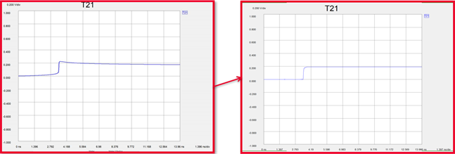
Time domain responses are most accurate closest to the location of the source. A discontinuity in the DUT will reflect some power back to the source, meaning less power is transmitted to the rest of the DUT. This loss of power going away from the source is referred to as masking, and allows the true impedance of the next discontinuity to be misrepresented.
The plot on the left shows the differential-mode input reflection of a device (SDD11). The first large discontinuity is the input connector; the second is the output connector. Because these connectors are physically identical, the apparent impedance difference between the two can be attributed to masking. The power level at the output connector has been decreased (masked) by the input connector. The plot on the right, output reflection (SDD22), proves this. Looking backwards into the device, the output connector now exhibits the greater apparent impedance. Were it not for masking, these two plots, and the measured impedance of the input and output connectors, would be identical.
The high dynamic range of a VNA-based PLTS system extends the ability of the instrument to accurately characterize devices that have several discontinuities or high loss. TDR-based PLTS systems may not be as accurate.
The response resolution describes how close in time two responses can be distinguished. This depends on the width of the impulse response, which is inversely related to the measurement bandwidth. The relationship between the three is approximately R = T = 1.25/BW; where R is the response resolution in picoseconds, T is the effective impulse width in picoseconds, and BW is the frequency span in GHz.
As described previously in Analyzing Time-Domain Signatures, the TDR signature provides specific circuit detail. Range resolution (TD span/Number of points, or Stop-Start/Number of points) will define how accurately the signature of a response can be identified. In general, a wider measurement bandwidth will provide finer spatial resolution.
To improve range resolution, zoom in on the section of interest and adjust the start- and stop-points to be as narrow as possible without compromising the agreement in the frequency domain.
When measuring short electrical devices, matching the spatial resolution to the minimum discontinuity distance is critical.
Impulse Response (IR) is the waveform that results at the output of a device when the input is excited by a unit impulse. As the maximum measurement frequency of a VNA increases, the pulse-width of the IR gets narrower. The pulse-width of the IR must be narrower than the two adjacent discontinuities in order to properly characterize the discontinuities in the time domain.
To illustrate this, assume we are measuring a device that has two discontinuities that are 1 cm apart and the expected response in the time-domain is as follows:
If the IR has a spatial resolution is greater than 1 cm and is swept across the DUT as shown below, the response in the time domain is dramatically different than what is expected. It looks like the picture on the right side of the illustration because the IR is larger than the two adjacent discontinuities, and the power levels from the multiple discontinuities are being added together.
The following shows the same device using an IR with a pulse-width that is less than 1 cm. The response you see in the time domain is much more like what is expected. It looks like the picture on the right side of the illustration. This is because the IR is narrower than the two adjacent discontinuities, and the IR is able to capture only the power level of the individual discontinuities.
Understanding the spatial resolution requirements of a device is extremely important as devices become shorter in length.
An increased number of points can help provide some additional resolution to data, but will never make up for using a system with insufficient spatial resolution. The following shows the same device but measured with the number of points set at 900 and at 4500. While there is some improvement, the improvement is not significantly better.
The idea to remember is that the spatial resolution of the PLTS system must be a narrower length than the expected minimum length of any adjacent discontinuities on the device.
When a measurement is made in the frequency domain and is converted to the time domain, the time domain start and stop frequencies can be ambiguous. This describes the algorithm for displaying the start and stop frequencies using the PLTS automated process.
This algorithm is best described using a flow diagram and a few examples of this process.
Automated Start and Stop Algorithm Flow Diagram
Parameter = SDD21 (Transmission)
Location of the SDD21 Peak Value in Time Domain = 2 ns
At Point 1,
Tstart = 0 ns
Tstop= 8 ns
The result is:
Tstart= 0 ns
Tstop= 8 ns
Parameter = SDD11 (Reflection)
Location of the SDD21 Peak Value in Time Domain = 2 ns
At Point 1,
Tstart = -1 ns
Tstop = 4 + 1 = 9 ns
The result is:
Tstart = -1 ns
Tstop = 4 + 1 = 9 ns
Parameter = SDD11 (Reflection)
Location of the SDD21 Peak Value in Time Domain = 5 ns
At Point 1,
Tstart =-2.5 ns
Tstop = 20 + 2.5 = 22.5 ns (greater than maximum time base of 10 ns)
At Point 2,
Tstart = -2.5 ns
Tstop = 10 - 2.5 = 7.5 ns
The result is:
Tstart = -2.5 ns
Tstop = 7.5 ns
The results in the start and stop calculations are not suitable to resolve the SDD21 with a 5 ns measurement. This is because the stop time is 7.5 ns while the device needs 10 ns for the two-way travel of in reflection. The system is capable of resolving 10 ns, however, due to the current calculation of the -2.5 ns start time, an artificial limitation has been imposed. This can be worked around by manually changing the start and stop in the gating mode.
Parameter = SDD11 (Any parameter)
Location of the SDD21 Peak Value in Time Domain = 0 ns
At Point 1,
Tstart = 0 ns
Tstop = 0 ns
At Point 3,
Tstart = -1 ns
Tstop = 1 ns
The result is:
Tstart = -1 ns
Tstop = 1 ns
Due to the absence of a strong signal in SDD21, the algorithm defaults to start of -1.0 ns and stop of 1.0 ns. This can be worked around by manually changing the start and stop in the gating mode.
The need for Time Domain Windowing is due to the abrupt Y-axis (magnitude) transitions in the Frequency Domain measurement at the Start and Stop frequencies. This band limiting of the frequency domain response causes overshoot and ringing in the Time Domain response. It causes the un-Windowed Impulse stimulus to have a sin (kt)/kt shape (k=p/frequency span), which has two effects that limit the usefulness of the Time Domain measurement:
Finite Impulse Width limits the ability to resolve between two closely spaced responses. The effects of the finite impulse width cannot be improved with increasing the frequency span of the measurement.
Impulse side lobes limit the dynamic range of the Time Domain measurement by hiding low-level responses within the side lobes of the higher-level responses. The effects of side lobes can be improved by windowing.
Windowing improves the dynamic range of the Time Domain measurement by modifying (filtering) the Frequency Domain data prior to conversion to the Time Domain to produce an impulse stimulus with lower side lobes. This greatly enhances the effectiveness in viewing Time Domain responses that are very different in magnitude. The side lobe reduction is achieved, however, as the trade-off with increased impulse width. The effect of windowing on the STEP stimulus is a reduction of overshoot and ringing while the trade-off is increased rise time.
The purpose of windowing is to make the Time Domain response more useful in isolating and identifying individual responses. The window does NOT affect the displayed Frequency Domain response. The windowing setting also has an effect on the transformation of eye diagrams.
The following shows typical effects of windowing on the Time Domain response of the reflection measurement of a short circuit.
Note: The various Window Types (Exponential, Kaiser, and so forth) can be used to increase and shift the range of these response times.
The following formula can be used to determine the equivalent 10 percent to 90 percent system rise time for the step function transformation and the eye diagram simulation:
Tr= (1000 / Fmax)¥RTEC
Where,
Tr = Rise time of the step response form 10% to 90% (in picoseconds)
1000 = Factor to convert frequency to picoseconds
Fmax= Maximum stop frequency used in the measurement (in GHz)
RTEC = Rise time equation coefficient
As an example:System rise time = 27 ps = (1000/ 20 GHz) ¥ 0.54 (see table below)
The following shows the equivalent rise times for a maximum frequency of 20 GHz for each window setting.
Window Selection |
TD Window Value1 |
Maximum |
Rise Time Equation Coefficient |
Equivalent |
|---|---|---|---|---|
Flat Response |
0.80 |
20 GHz |
0.91 |
45.5 ps |
Nominal |
0.50 |
20 GHz |
0.71 |
35.5 ps |
Fast Rise Time |
0.20 |
20 GHz |
0.54 |
27 ps |
1 The relationship between the TD window value and the rise time equation coefficient is not made available.
By increasing or decreasing the filter value above or below the default, a trade-off can be made between rise time and side-lobe level (dynamic range).
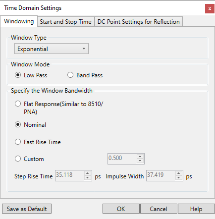
When Time Domain Settings is selected from the Tools menu, the Time Domain Settings dialog box is displayed allowing a choice of the three Time Domain Window settings.
The previously-selected window settings are used whenever you open measurement data in time domain format.
Click Tools, then Time Domain Settings
Then select from: Windowing, Start and Stop time, DC Point Settings
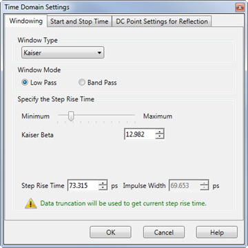
Windowing Tab
Window TypeThe Window Type setting can be used to change and shift the range of the Step Rise Time and Impulse Width settings shown at the bottom of the Windowing tab. Choose from the following:
Window ModeAll Time Domain measurements are made in the Frequency Domain. Using Inverse Fast Fourier Transform (IFFT), the time and distance measurements are calculated.
Window Bandwidth
Learn how to change between Impulse and Step stimulus. You can set a User Preference for the default Step Rise Time calculation from 10-90% to 20-80%. Learn more. Beginning with PLTS 2018, Kaiser windowing allows system rise times to be set to slower settings than in previous versions of PLTS. If the step rise time is set to be slower than the response of the filter based on the current frequency settings, Data truncation will be used to get current step rise time is displayed indicating that data has been truncated. For slower rise times, only a portion of the entire range of frequency data is used to compute the time domain in order to obtain the desired step rise time setting. The frequency data is not changed.
Save As DefaultClick this button to save the new settings as default. PLTS will use the saved settings as default to calculate time domain parameters when users import/open new data file. |
||||||||||||||||||
Start and Stop Time Settings
This dialog allows you to change and view the start times and stop times of time domain plots three ways. Note: The feature is used only for frequency domain S-parameter files that are calculated to show time domain. If your measurement was taken using a TDR, this feature does not apply. How to launch the Start and Stop time settings: Click Tools, then Time Domain Settings,thenStart and Stop Time. You can make changes, then see the changes in the main PLTS window without closing the dialog box.
Auto Optimize Off or Auto Optimize On The default for this setting can be made on the Measurement tab or the User Preferences dialog.
All differential and single-ended time domain parameters are placed in the Available Parameter List. Move the parameters that have a start or stop time that you would like to change to the Selected Parameter List. using the eight Move Parameters Buttons located between the two lists.
Once the parameters are listed in the Selected Parameter List, change the Start Time and the Stop Time using the Start Time and the Stop Time text entry boxes. The times can be changed two ways:
Note: The spinners increment or decrement only the most significant digit that was highlighted with the mouse. For example, the Stop Time in the above graphic is 5.34 ns. If you highlight the entire "5.34" value or just the "5", clicking the up spinner increments the "5". However, if you highlight the "34" or only the "3", clicking the up spinner increments the "3". |
||||||||||||||||||
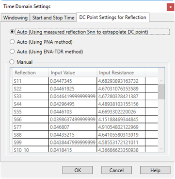
DC Point Setting for Reflection (Measurements)When using a VNA, measurements are made in the frequency domain and transformed to the Time Domain. These frequency domain measurements are limited by the low frequency range of the VNA, typically about 10 MHz.
Auto (Default) PLTS uses a linear extrapolation algorithm to determine DC point from the measured values. This choice may not yield the best results when the reflection return loss is -30 dB or lower. Auto Using PNA method The PNA uses a circle extrapolation algorithm to determine DC point from the measured values. Use this choice when the return loss from a reflection measurement is -30 dB or lower. Auto Using ENA-TDR method Uses ENA with the TDR option to compute DC point. Manual Change DC point value, or corresponding resistance value, for reflection S-parameters to manually adjust the slope of the corresponding time domain parameters.
|
||||||||||||||||||
Optimize Time Domain Transformation for Data File with DC Values Beginning with PLTS2021, DC values when transforming to the time domain are removed automatically. This enhances high frequency extrapolation accuracy.
|
You can measure the rise time of traces in a plot.
Rise Time is calculated as follows:
The Y-axis Min and Max values are found and the difference between the two is calculated.
A marker is placed at the 10% value, and another at the 90% value.
The X-axis delta between the two markers is displayed as Rise Time.
You can set a User Preference to change the percentages to 20% - 80%.
How to measure Rise Time.
Right click in the plot, then click Measure, then Step Rise Time
Check Rise Time measurement ON to enable and disable a Rise Time (Tr) measurement.
Select either:
Measure rise time trace Select a trace for which rise time is to be measured and displayed.
Measure maximum rise time of all traces Finds and displays the maximum rise time of all of the displayed traces.
Check Rise Time limit and enter a value. The measured rise time is compared to this value.
If the displayed rise time is HIGHER than the entered value, FAIL is displayed with the rise time value.
If the displayed rise time is LOWER than the entered value, PASS is displayed with the rise time value.
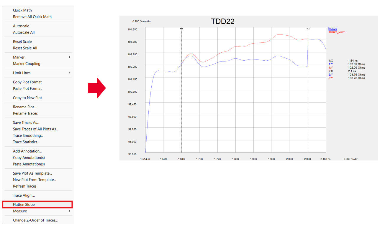
This feature supports flattening the TDR impedance slope according to the requirement of TC9.
Right click in the plot, then click Flatten Slope.
The software automatically displays two markers, and the data between them will be flattened.
Drag the two markers to adjust the start and stop points for flattening.
With two or more traces present in a plot, you can automatically measure the skew between the traces.
Beginning with PLTS 2013, Skew is calculated using Step stimulus (formerly Impulse) resulting in better accuracy. In addition, Skew can be measured as a percentage of amplitude or at an absolute voltage level.
Skew between two traces is calculated as follows:
Markers are placed at the specified location on each trace.
The X-axis delta between the two markers is displayed as Skew.
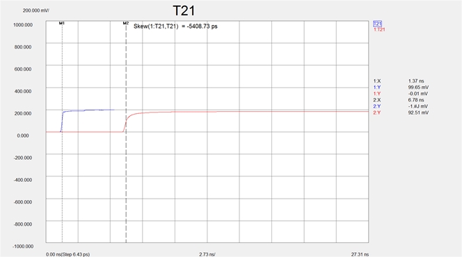
Skew values are relative to the first trace. A negative value indicates that the second trace is longer than the first trace; a positive value indicates that the second trace is shorter than the first trace. The following plot shows a negative skew value.
How to measure Skew.
With two or more traces present in a Time Domain differential or single-ended view: (Learn how to add traces to a plot), right click in the plot, then click Measure, then Skew.
Check Skew measurement ON to enable and disable a skew measurement.
Measure skew of trace Select two traces for which skew is to be measured and displayed.
Measure maximum skew of all traces Finds and displays the maximum skew between the fastest and the slowest of the displayed traces.
In the skew measurement, we use two markers to find the target amplitudes on the two step responses.
Percentage of amplitude The percentage of the displayed amplitude of each trace at which to position the two markers. In the following plot, 50% is used.
Voltage The absolute voltage value of each trace to position the two markers. In the following plot, 100 mv would have yielded the same result.
Check Skew limit and enter a value. The measured skew is compared to this value.
If the displayed skew is HIGHER than the entered value, FAIL is displayed with the Skew value.
If the displayed skew is LOWER than the entered value, PASS is displayed with the Skew value.
Skew Measurement using 50% Reference
Two TDR traces can be aligned using the Trace Align feature:
Right-click on a plot then select Trace
Align....
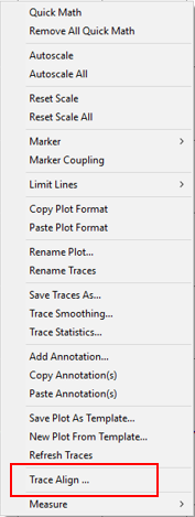
The Trace Align...
dialog is displayed:
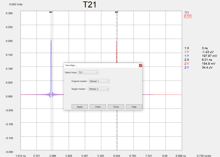
Select the desired trace using the Select trace pull down menu.
Select the original marker using the Original marker pull down menu. This is the trace that will be moved and aligned with the Target marker.
Select the target marker using the Target marker pull down menu.
Click on the Apply
button to align the two traces.
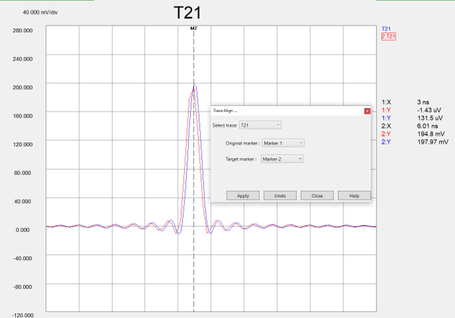
Click on the Undo button to undo the trace alignment.
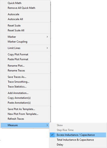
How to measure excess inductance and capacitance
Right click on a plot, then click Measure,
then Excess Inductance / Capacitance.
Two markers will be added to the plot.
Drag the two markers to where you want to measure the excess.
A drag-able label reports the excess between the markers.
To turn the markers OFF, right click on a TDR plot, then click Measure, then Excess Inductance / Capacitance.
The format must be impedance.
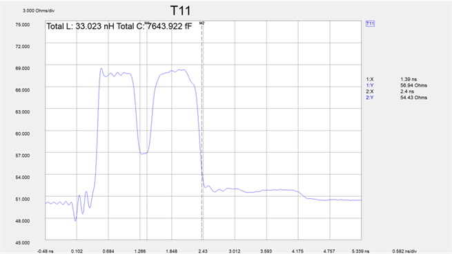
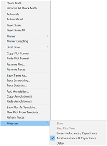
How to measure total inductance and total capacitance
Right click on a plot, then click Measure,
then Total Inductance & Capacitance.
Two markers will be added to the plot.
Drag the two markers to where you want to measure the totals.
A drag-able label reports the totals between the markers. Positive amplitude is reported as inductive reactance in nanohenries (nH). Negative amplitude is reported as capacitive reactance in femtofarads (fF)
To turn the total markers OFF, right click on a TDR plot, then click Measure, then Total Inductance & Capacitance.
When viewing the time domain response of a test device that has multiple discontinuities, energy is reflected, and then re-reflected. Finding the exact location of the discontinuities is very difficult, especially in low-loss devices.
The Correct Impedance Profile feature invokes an algorithm which corrects for the energy re-reflected from multiple discontinuities. This can be helpful when trying to identify the exact location and signature of discontinuities in a low-loss device.
How to set Correct Impedance Profile
Click Tools, then Correct Impedance Profile
When Correct Impedance Profile is ON (checked), all REFLECTION plots that are viewed in Time Domain are displayed with a yellow icon in the upper right corner as shown below.
During a Time Domain measurement, one of the following may appear in the corner of the display. Learn more about these icons.
Icon |
Icon Name |
|---|---|
|
Resampled Data - This icon indicates that only the harmonically-related data points were used to generate time domain data. |
|
Interpolated Data - This icon indicates interpolation is performed to calculate the harmonically-related points that were not measured. Any measurements that were performed at harmonically-related points are left unchanged. The interpolated data is used, along with the measured harmonically-related data, to perform the Inverse Fast Fourier Transform (IFFT) for the calculated time domain data. |
|
Bad Data- This icon indicates there are less than 10 harmonically-related data points in the measured data. In this case, all of the non harmonically-related data is used to perform the Inverse Fast Fourier Transform (IFFT) to calculate time domain data. This may result in inaccurate time domain data. |
There are a number of practical considerations in examining time domain data, as described previously. Therefore, it is very important to have a method of validating the data. This can be accomplished by comparing the original frequency domain data to the data after it is inverse Fourier transformed into the time domain, and then Fourier transformed back into the frequency domain, as shown below. Ideally, these data should be identical. Changing the time domain start and stop points, the filter value, and the value of the DC parameter may improve the agreement.