Trace Math

Math may be performed on traces that are displayed within a plot. For example, you may divide the data of one trace by the data of a second trace to derive the vectorial difference.

The following two methods can be used to perform Trace Math:

Create and apply a Math Equation to a displayed plot or trace.
Perform Quick Math on a displayed trace.

Math equations can be saved and applied to templates. However, templates can use math equations that include data ONLY from the same file, such as “1:S11 / 1:S22”. Equations from multiple data files (such as “1:S11 / 2:S11”) are NOT supported in templates.

Other Analysis Tools and Utilities Topics

How to Create a Math Equation

Click Tools, then Math, then Design
Enter an equation using the Data, Key Pad, and Functions buttons.
When finished, type a new Equation Name or select an existing Equation Name to overwrite.
Click Save Equation. The equation is now resident in PLTS memory. It can now be Applied to plots of the same data analysis type.
Optional: click Save Advanced to save the equation to a *.DUT file or a *.fml file on your PC. Learn more.

Important Note:

Use this dialog to create, load, and save math equations.

When you Save or Load an equation, it becomes resident in PLTS memory.

You can then Apply that equation to a plot of the same Data Analysis type.

The equation remains resident in memory until PLTS is closed or the equation is deleted.

Beginning with PLTS 4.5, you can Save and then Recall a math equation with a *.DUT file or an equation (*.fml) file.

Learn how to Add an Equation trace to a plot.

Create Equations dialog box help

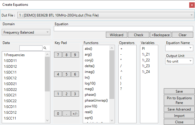
DUT File - Choose an open data file to include in the math operation. Data from up to three different files may be used in an equation.

Domain - Choose the data to display and include in the math operation. Select from Frequency Domain (single-ended and balanced) and Time Domain (single-ended and differential).

Data - Click a parameter and it is copied to the cursor location in the equation. Use the search filter text box to do a quick search of the data list.

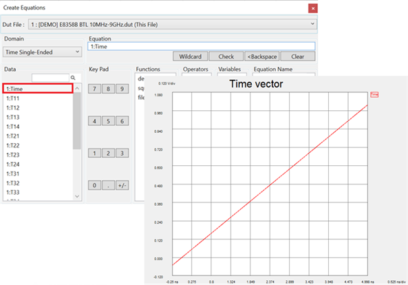
Time Vector - Beginning with PLTS 2022, time vector is available for standard, MATLAB, and Python equations:

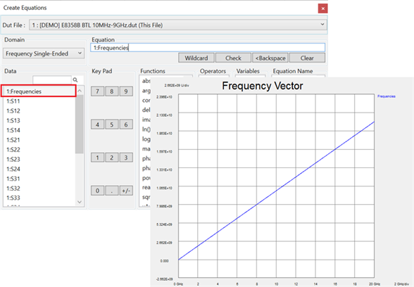
Frequency Vector - Beginning with PLTS 2022, frequency vector is available for standard, MATLAB, and Python equations:

Equation - Build the equation using Data, Functions, Operators, Variables, and the Key Pad.

Key Pad - Used to build the equation. It allows you to enter numeric entries and operators.

New Wildcard - When clicked, replaces the DUT designators in the formula with '?'. When the equation is applied, the wildcard is replaced with the number of the first open DUT file with the matching parameter. Using the wildcard will usually avoid the need to resolve ambiguity in a formula. Use a wildcard ONLY when you know which parameters will be matched.

Check - When the equation is complete, click to check the syntax of the equation. Red text appears when the equation has an error (as in the above image). No red text means that the equation is valid.

Equation Name - Allows you to enter a name to save the equation and recall it for future use.

Output Unit - Set the output units to No unit, Ohms, or dB. The units are applicable for PLTS as well as third-party Matlab/Python equations. If adding the impedance equation to a new plot, |Z| is displayed by default. If adding the impedance equation to an existing plot for data sharing, the plot format must be related to impedance.

Save (Equation) Saves the valid math equation into PLTS memory. NOTE: This does NOT save the equation to disk.

The following two buttons replace each other depending on the current 'pin' state.

Pin to Equations Pane The current (unpinned) equation is pinned to the Equations Pane.

Unpin from Equations Pane The current (pinned) equation is unpinned from the Equations Pane.

Save Advanced Launches the Save Equations dialog, which allows you to save the equation to a *.DUT file or a *.fml (equation) file.

Load Launches a Open dialog. Navigate and select a *.fml (equation) file to load. After opening the file, select the file using equation Name.

Close Closes the dialog.

Variables - Beginning with PLTS 2020, the port impedances Z1, Z2, ...Zn have been added as variables and they do not have to be 50 ohms. The port impedance variables are available for both frequency-domain and time-domain equations.

Functions - Used to build the equation. It allows you to enter math symbols and delimiters as well as some frequency domain formats.

Abs ( ) - Returns the absolute value of the following term. Not available for Time Domain.
Arg ( ) - Returns the standard argument function for complex numbers. Not available for Time Domain.
Conj ( ) - Returns the standard conjugate function for complex numbers. Not available for Time Domain.
Delta ( ) - Returns the difference (D) of the following terms.
Imag ( ) - Returns the imaginary portion of the following complex term. Not available for Time Domain.
Ln(ComplexArray a) - Returns the natural logarithm (base e logarithm) of complex numbers. Not available for Time Domain.
Log10(ComplexArray a) - Returns the base 10 logarithm of complex numbers. Not available for Time Domain.
Mag(ComplexArray a) - Same as “abs()” Extracts the modulus of complex numbers, equal to sqrt(a.re*a.re+a.im*a.im). Not available for Time Domain.
Phase(ComplexArray a) - Returns the phase (in degrees) of a trace. The result must be viewed in Real format. Not available for Time Domain traces.
PhaseUnwrap(ComplexArray a) - Same as phase, but not wrapped at 180°. The result must be viewed in Real format. Not available for Time Domain traces. See Create Phase Equation Example.
Pow10(ComplexArray a) - Raise base 10 to the power of another complex number. Not available for Time Domain.
Real ( ) - Returns the real portion of the following complex term. Not available for Time Domain.
Sqrt ( ) - Returns the square root of the following term.
XAxisIndex( ) - Returns the current index in the sweep.
XAxisValue( ) - Returns the current value of the x-axis index.
getNumOfPoints( ) - Returns the number of points for a trace.
fileSum( ) - Sum the data for a collection of parameters. The collection is comprised of all open views or multi-data templates. For example: fileSum(1:S11) will sum the S11 parameter for all of the open views. The "1:" is ignored.
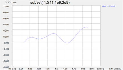
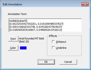
subset(,,) - Allows start and stop equation limits in the frequency domain. The first parameter is the S parameter. The second parameter is the start frequency and the third parameter is the stop frequency. For example, subset(1:S11,1e9,2e9).

Save Equations Dialog

The following dialog is launched by clicking Save Advanced on the Create Equation and Apply Equation dialogs.

Save Equations dialog box help

The equations that are in PLTS memory are listed.

Check the equations to be saved, then click either Save in Active DUT file, or Export to Equation File.

Check All Selects all displayed equations.

Clear All Unchecks all checked equations.

Save in Active DUT file When the DUT file is loaded, the equation is also recalled into PLTS memory.

Export to Equation File This file can be recalled and used with any active DUT file.

Applying a Math Equation

Once math equations have been created and saved (learn how), they may be applied ONLY to the same Data Analysis type for all opened data files. For example, a Single-ended Frequency domain equation can be applied ONLY to a Single-ended Frequency domain plot. Otherwise, the Apply menu selection is not available.

Learn how to Add an Equation trace to a plot.

How to Apply a Math Equation

Click Tools, then Math, then Apply
Select an equation to apply to the active trace.
Click Apply to Trace

Choose Equation Traces to Display dialog box help

Important: Only the equations that were created using the same Data Analysis type as is the currently-active trace appear in the dialog and can be applied. For example, if MyNewEquation was created in Time Domain (Single-ended), then that equation appears ONLY when the active trace is Time Domain (Single-ended).

The first three equations that appear (Upper Std Dev, Mean, Lower Std Dev) are standard PLTS Statistical Equations. Learn more.

Apply to Trace Adds a new math trace to the active plot.

Apply to Text Box Adds equation results to the active plot.

After selecting an equation and clicking the Apply to Text Box button, the equation results are displayed on the plot. An example is shown below:

Right-click on the text box to edit the annotation:

Remove Trace Removes the math trace from the plot.

Remove Text Box Deletes equation results from the active plot.

Delete Deletes the selected equation from PLTS memory.

The following two buttons replace each other depending on the current 'pin' state.

Pin to Equations Pane The selected (unpinned) equation is pinned to the Equations Pane.

Unpin ALL from Equations Pane Unpins all equations from the Equations Pane.

Save Advanced Starts the Save Equations dialog.

Import Recalls equations that are stored in a *.fml file.

Exit Closes the dialog box.

Resolve Data Ambiguity dialog box help

When applying an equation, this dialog appears when the files to which the equation refers is ambiguous. This occurs because the files that are open may NOT be the same files that were open when the equation was created.

The files are identified by the numeric prefix before each term and each open file. For example (from the above dialog image): with 1:S11, the '1:' file MAY NOT be the same '1:' file that was open when the equation was created. Please confirm the '1:' file to use by using the following procedure:

In the left pane, click the equation reference to be resolved.
In the right pane, click the file to associate with that equation reference.
Click <<
Continue until all equation references are resolved.
When finished, click Apply

When applying this equation during the current PLTS session, always resolve ambiguities using the current active file.

Check this box to always use the ACTIVE (selected) file in the equation.

Leave cleared to manually resolve ambiguities.

Cancel Do NOT apply this equation. Other equations that may be loading will be applied or prompt for resolution.

Using Quick Math

You can use Quick Math to perform simple math operations on two traces in the same plot. The resultant trace is displayed on the plot.

How to perform a quick math function

With MORE THAN ONE data trace displayed on the active plot, click the right mouse button with the cursor over the plot. Then click Quick Math.

In the Left Operand field, select a trace on which math is to be performed.
In the Operator field, select an operation (+ add, - subtract, * multiply, / divide).
In the Right Operand field, select a second trace on which math is to be performed.
Click Result (=) to add a new math trace to the active plot.

Right-click the plot, then Remove All Quick Math to remove the math trace.

Export Data with Applied Math

Beginning with PLTS Release 4.2, data can be exported with Math applied. Learn more.

Last Modified:

16 Jan 2024	The Output Unit drop-down menu now supports dB
1-Dec-2021	Added Time and Frequency Vector data
11-Nov-2019	Added data search filter text box and output unit functions to Create Equation dialog descriptions
7-Jan-2013	Added new functions (2013)
7-Nov-2011	Edited Apply and Quick math for 2012
1-Mar-2011	Updated for 2011
3-Apr-2008	Added Save math equations