RJ Compensation

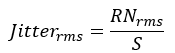
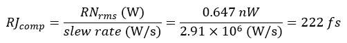
The random noise (RN) of a receiver can influence the jitter result when the input power level approaches the noise floor for a given receiver. A signal's slew rate is an important factor in determining how much noise is converted into jitter. The following equation shows the relationship between RN and jitter, where S is the slew rate in W/s.

Optical signals are particularly susceptible to noise, and an increase in noise may negatively influence jitter analysis results when operating near the noise floor of an optical receiver, such as a 86100D plug-in module.

Important Points Learned in this Topic

• FlexDCA Option 200 provides RJ/RN compensation, which can be used to remove the influence of noise from the jitter result. This is accomplished in four steps:
1. Measure optical module noise floor
2. Determine slew rate for signal
3. Calculate amplitude noise contribution to timing jitter
4. Enter this result as the RJ compensation, RJ_comp, value
• As RJ_comp increases for lower optical power levels, the uncertainty in the final result also increases. In other words, a small change in RJ_comp can result in a large change in the final RJ value result. In practice, this approach is feasible when RJ_comp is smaller than RJ_final as shown in the graph at the end of this topic.
• The slew rate (W/s) is a function of the optical power level and needs to be measured for the specific signal under test at the current optical power level.

Procedure

This process removes the RN contribution from the measured jitter.

Measure Module's Optical Noise Floor

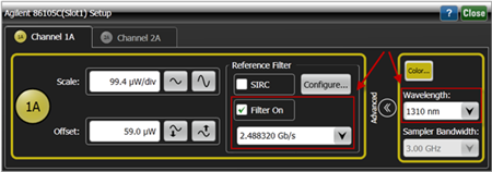
Measure module noise floor with compliance filter active and no input signal. It is important to make sure the module noise floor is measured with the wavelength set appropriately and with the compliance filter enabled for the symbol rate of interest.

1. Place FlexDCA in Eye/Mask mode.
2. Disconnect any input signal from the 86100D input channel that you are using. In FlexDCA, open the Channel Setup dialog. (Click Setup > Modules > Channel N.)
3. Enter the wavelength and select the compliance filter for the symbol rate of interest.



4. Click Measure > Histograms. In the Histograms dialog, turn on Histogram 1 which is a default vertical histogram.
5. Close the Histogram dialog.
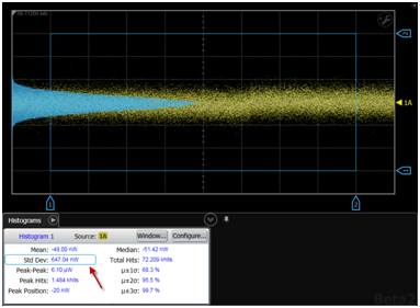
6. In the Histograms results table, locate the standard deviation listing as shown in the following figure. The histogram's standard deviation is the module's noise floor which you'll use later in this procedure.

Measure Slew Rate

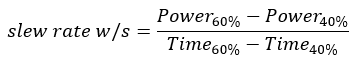
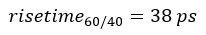
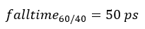
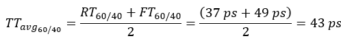
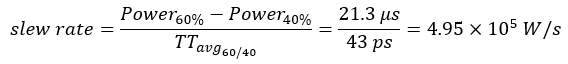
The slew rate is calculated from the transition time and power level as shown in the following equation:

7. Connect your signal to the module's channel input.
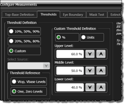
8. Click Measure > Configure Base Measurements. In the dialog, select the Thresholds tab.
9. In the Threshold Definition field, select Custom.
10. In the Custom Threshold Definition field, enter 60% upper, 50% middle, and 40% lower level threshold definitions.
11. In the Threshold Reference field, select One, Zero Levels as shown in the following dialog.



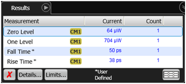
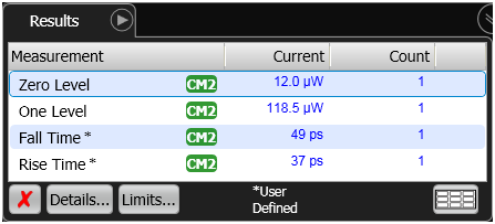
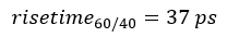
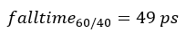
12. On the signal, measure Fall Time, Rise Time, Zero Level, and One Level. From these measurements, calculate the slew rate as shown for the following example. The example is an eye diagram for an optical transmitter with −4.00 dBm output power and the results shown in the following figure.

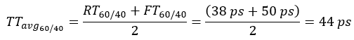
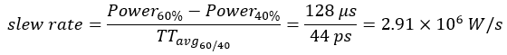
Passing the same optical transmitter signal through an attenuator results in an optical power of −12.0 dBm and the results shown in the following picture. The slew rate in this instance is calculated as follows:

Calculate the Noise Contribution to Jitter, RJ_comp

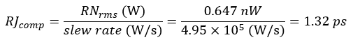
13. Now that the module's noise floor and slew rate have been measured, calculate the contribution of noise to jitter, RJ_comp. Divide the module's noise floor measured above by the slew rate calculated in the previous step.

In the example with the higher power optical signal, the RJ_comp is small, 222 fs, because the input optical power is much larger than the module's noise floor.

However, as the optical power is reduced and approaches the noise floor of the module, the RJ_comp increases to 1.31 ps.

Comparing the jitter mode results for the different power levels, the impact of RJ_comp on the measured random jitter becomes clear. The larger input power has a random jitter of 1.35 ps while the lower optical power has a random jitter of 1.83 ps. These results include the contribution of both jitter and noise.

Enter RJ_amp as the RJ Compensation Value

FlexDCA's RJ/RN compensation allows you to enter a RJ level which is removed from the measurement.

14. Place FlexDCA in Jitter/Noise mode.
15. Click Measure > Configure Jitter Mode Measurements to open the Configure Jitter Mode Measurements dialog.
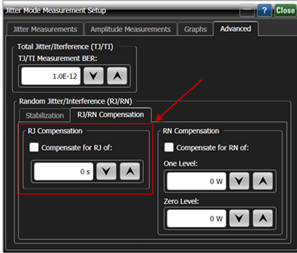
16. In the dialog, select the Advanced tab. Within the Advanced tab select the RJ/RN Compensation tab.
17. Enter the noise contribution to the jitter, RJ_comp, previously calculated as into the dialog and select Compensate for RJ of:.

After entering the RJ/RN compensation values for the two different optical power levels the reported RJ for both cases is similar. The RJ reported for the high power optical input is 1.33 ps, while the value reported for the low power input is 1.285 ps.

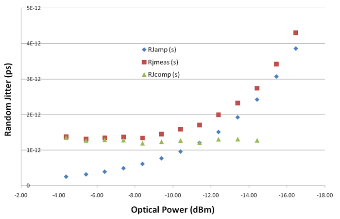
The following plot shows the RJ from the same optical source measured using an 86105C module versus power level. Once the noise contribution to jitter is removed, the RJ remains constant as the optical power is reduced as shown by the green symbols.