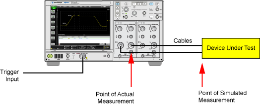
Studying this example provides the easiest way to learn how to use the DeEmbedding operator. After learning about this simple case, you should be able to progress to more advanced models. These steps show how to remove the insertion loss of a cable. If we cannot connect the 86100D directly to the two-port DUT (Device-Under-Test), we must connect two cables between the 86100D and the DUT. We actually end up measuring what the signal looks like after the signal has passed through the cables. Removing the insertion loss of both cables simulates the measurement at the DUT. Let us assume we measured each cable's S-parameters using an 86100D with a 54754A TDR/TDT module, and the S-parameters are saved to two files (.s2p).

1. Drag the DeEmbedding operator into the construction area. If the symbols for the input channels are not located on the operator's inputs, drag the channel symbols from the Inputs panel to the operator's inputs.



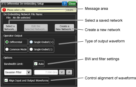
2. Click on the operator to open the DeEmbedding Setup dialog.

"Please select a file" message. This note (at the top of the dialog box) alerts you that you have previously defined your setup in a transfer function file (*.tf2), you can click Select a Network to open your file. In this example, the remaining steps will create the transfer function file.


3. Select the Operator Output as Single Ended (+).
4. Click Create a New Network and the DeEmbedding Network Setup dialog opens as shown in the following figure. In this dialog, the values highlighted in blue define the measurement circuit and node while the values in bronze define the simulation circuit and node. Notice the Transmitter, Channel, and Scope blocks in this interactive diagram. Later in this procedure you will click on these components to configure them.



Please select a file message. This note alerts you that the Channel block is currently defined by a file. This will be addressed later in this procedure.

Refer to Transform Function Messages if a warning message is displayed while creating a new network.

Network Blocks

In the preset configuration network diagram, the various blocks model components such as cable loss, probe loading, or a fixture. The default name (for example, the Channel A block shown here), indicate a typical use depending upon the chosen preset. This is a convenience for referring to blocks and an example of how the block may be used. However, you can define them any way you like. While these blocks represent different parts of the circuit, they have the exact same definition selection to choose from. Their names simply help you understand what they might represent in your circuit.

5. From the Preset Configuration drop-down list, select Remove insertion loss of a fixture or cable from the following choices:
• Remove insertion loss of a fixture or cable
• Add insertion loss of a fixture or cable
• Remove scope input relection
• Remove all effects of a fixture or cable
• Add all effects of a fixture or cable
• Replace one channel element with another
• Relocate the observation node of a measurement
• Remove all effects of a probe
• Remove loading effects of a probe
• Relocate the observation node of a probed measurement
• General purpose probe
• General purpose 6- and 9- block topologies with user defined measurement and simulation points.

With the General purpose 6- and 9- block topologies, each block can be defined as having a combination of up to three elements in cascade, series, or parallel arrangements giving you 27 total possible circuit elements to define for the most sophisticated scenarios. For SMA differential probe usage, the general purpose 6- block model will find use in the majority of cases. For those very sophisticated applications (for example, using both high impedance probes and differential SMA probe heads) the general purpose model can be used to describe these complex cases.

6. Click the Transmitter block to open the Transmitter Impedance Setup dialog. Enter the impedance values for both Measurement and Simulation circuits and close the dialog. The default value is 50 ohms.



7. Click the Scope block to open the Receiver Impedance Setup dialog. Enter the impedance values for both Measurement and Simulation circuits and close the dialog. The default value is 50 ohms.
8. Click the Channel block to open the Channel Setup dialog. From the drop-down list, select the Circuit Block Type. The following choices are available to define the Circuit Block Types. For this example, in the Simulation Circuit tab confirm that Thru is selected.
• Thru
• Open
• File. Defines a model block using standard 4-port S-parameters. Using full 4-port S-parameter models is often necessary because cross-coupling components are included between all four ports in the model. However, it is sometimes more convenient to split the 4-port model into two uncoupled 2-port models, as described in the following two selections.
• Dual 2-Port. Defines a model block using two standard 2-port model blocks. One block defines the path between ports 1 and 2 and one block for the path between ports 3 and 4. For example, two 2-port S-parameter files can model a pair of coaxial cables. Or, when you have an accurate s-parameter file for the differential path through a device, but not for the common mode path. You can use a 2-port differential S-parameter file to model the differential path and an RLC block to model the common mode path. In this case, you define each 2-port block type independently to be a Thru, Open, RLC, Lossless Transmission Line, 4-Port S-Parameter File, or Combination of 4-Port Sub-Circuits.
• Dual 2-Port Mixed Mode. Defines a model block using two 2-port differential model blocks (one for the differential path and one for the common-mode path). You can define the 4-port model block as a combination of two different uncoupled 2-port model blocks. One block is for the differential path through the device and one block for the common mode path through the device. In this case, you define each 2-port Block Type independently to be a Thru, Open, RLC, Lossless Transmission Line, 4-Port S-Parameter File, or Combination of 4-Port Sub-Circuits.
• Combination of Subcircuits

For the simulation we want to perform, the block needs to be defined as a Thru, meaning that the block acts as though it is not there. Remember in the measurement circuit that we had the signal exiting the DUT, passing through the cable, and entering the oscilloscope. We could only measure it at the front end of the oscilloscope. We actually wished we could have measured the signal before it entered the cable so we could remove any loss induced by the cable.

9. In the Measurement Circuit tab, select Dual 2-Port.
10. In the Port 1-2 Block Setup tab, select File for the Circuit Block Type.
11. Click Browse and import the S-parameter file for the cable that is connected to channel 1A.
12. In the Port 3-4 Block Setup tab, select File for the Circuit Block Type.
13. Click Browse and import the S-parameter file for the cable that is connected to channel 2A.

Since the S-parameters represent a cable, S21 = S12, selecting Flip Model and 4 Port Numbering will have no effect.

14. Close the Channel Setup dialog.
15. In the De-Embedding Network Setup dialog, click Save As to save the network setup as a transfer function file (*.tf4). Close the dialog.

When creating detailed setups, click Save As when you begin creating your setup and click Save often as you progress. This will protect you from accidental data loss in case of a problem.

You must save your setup to a file before it can be used.



16. The application automatically sets the bandwidth limit. You can manually set the bandwidth limiting to minimize effects caused by noise that occurs above the frequency where the signal is mostly attenuated.
17. Measurements are now simulated at the input to the DUT.